ESSENTIAL STATISTICS 2 E William Navidi and Barry

ESSENTIAL STATISTICS 2 E William Navidi and Barry Monk ©Mc. Graw-Hill Education. All rights reserved. Authorized only for instructor use in the classroom. No reproduction or further distribution permitted without the prior written consent of Mc. Graw-Hill Education.

Frequency Distributions and Their Graphs Section 2. 2 ©Mc. Graw-Hill Education.

Objectives 1. Construct frequency distributions for quantitative data 2. Construct histograms 3. Determine the shape of a distribution from a histogram ©Mc. Graw-Hill Education.

Objective 1 Construct frequency distributions for quantitative data ©Mc. Graw-Hill Education.

Frequency Distribution for Quantitative Data To summarize quantitative data, we use a frequency distribution just like those for qualitative data. However, since these data have no natural categories, we divide the data into classes. Classes are intervals of equal width that cover all values that are observed in the data set. The lower class limit of a class is the smallest value that can appear in that class. The upper class limit of a class is the largest value that can appear in that class. The class width is the difference between consecutive lower class limits. ©Mc. Graw-Hill Education.

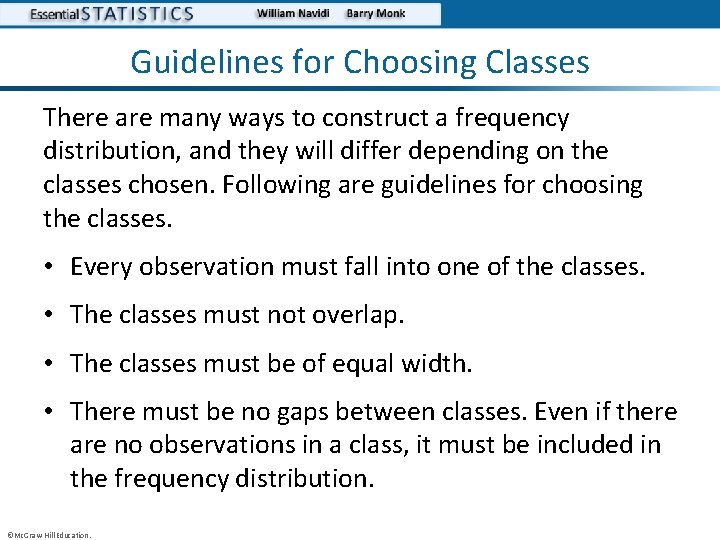
Guidelines for Choosing Classes There are many ways to construct a frequency distribution, and they will differ depending on the classes chosen. Following are guidelines for choosing the classes. • Every observation must fall into one of the classes. • The classes must not overlap. • The classes must be of equal width. • There must be no gaps between classes. Even if there are no observations in a class, it must be included in the frequency distribution. ©Mc. Graw-Hill Education.

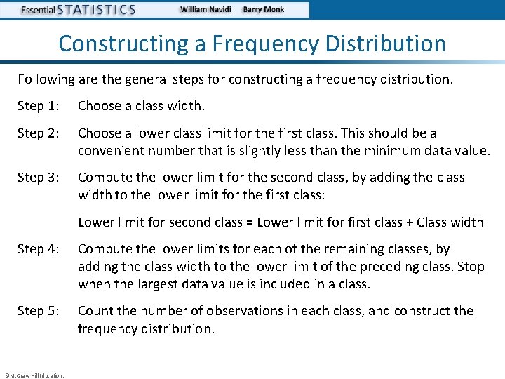
Constructing a Frequency Distribution Following are the general steps for constructing a frequency distribution. Step 1: Choose a class width. Step 2: Choose a lower class limit for the first class. This should be a convenient number that is slightly less than the minimum data value. Step 3: Compute the lower limit for the second class, by adding the class width to the lower limit for the first class: Lower limit for second class = Lower limit for first class + Class width Step 4: Compute the lower limits for each of the remaining classes, by adding the class width to the lower limit of the preceding class. Stop when the largest data value is included in a class. Step 5: Count the number of observations in each class, and construct the frequency distribution. ©Mc. Graw-Hill Education.

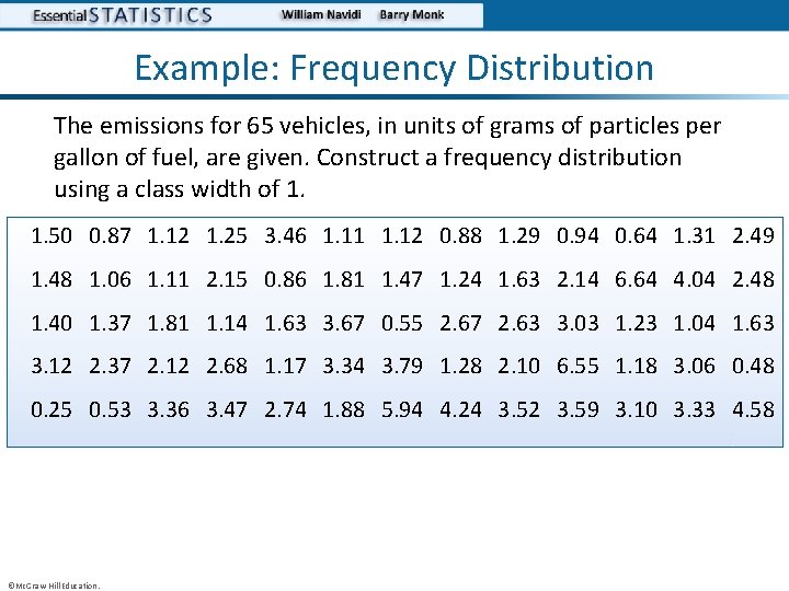
Example: Frequency Distribution The emissions for 65 vehicles, in units of grams of particles per gallon of fuel, are given. Construct a frequency distribution using a class width of 1. 1. 50 0. 87 1. 12 1. 25 3. 46 1. 11 1. 12 0. 88 1. 29 0. 94 0. 64 1. 31 2. 49 1. 48 1. 06 1. 11 2. 15 0. 86 1. 81 1. 47 1. 24 1. 63 2. 14 6. 64 4. 04 2. 48 1. 40 1. 37 1. 81 1. 14 1. 63 3. 67 0. 55 2. 67 2. 63 3. 03 1. 23 1. 04 1. 63 3. 12 2. 37 2. 12 2. 68 1. 17 3. 34 3. 79 1. 28 2. 10 6. 55 1. 18 3. 06 0. 48 0. 25 0. 53 3. 36 3. 47 2. 74 1. 88 5. 94 4. 24 3. 52 3. 59 3. 10 3. 33 4. 58 ©Mc. Graw-Hill Education.

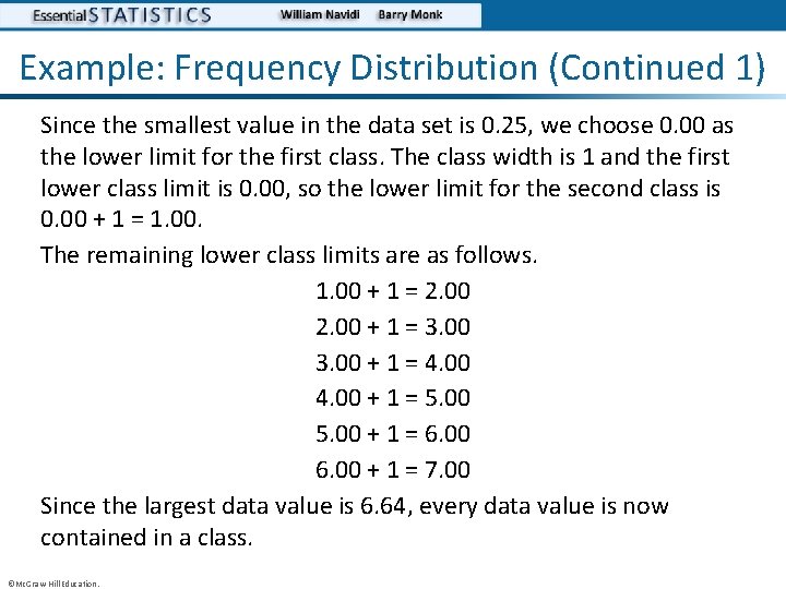
Example: Frequency Distribution (Continued 1) Since the smallest value in the data set is 0. 25, we choose 0. 00 as the lower limit for the first class. The class width is 1 and the first lower class limit is 0. 00, so the lower limit for the second class is 0. 00 + 1 = 1. 00. The remaining lower class limits are as follows. 1. 00 + 1 = 2. 00 + 1 = 3. 00 + 1 = 4. 00 + 1 = 5. 00 + 1 = 6. 00 + 1 = 7. 00 Since the largest data value is 6. 64, every data value is now contained in a class. ©Mc. Graw-Hill Education.

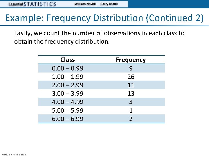
Example: Frequency Distribution (Continued 2) Lastly, we count the number of observations in each class to obtain the frequency distribution. Class 0. 00 – 0. 99 1. 00 – 1. 99 2. 00 – 2. 99 3. 00 – 3. 99 4. 00 – 4. 99 5. 00 – 5. 99 6. 00 – 6. 99 ©Mc. Graw-Hill Education. Frequency 9 26 11 13 3 1 2

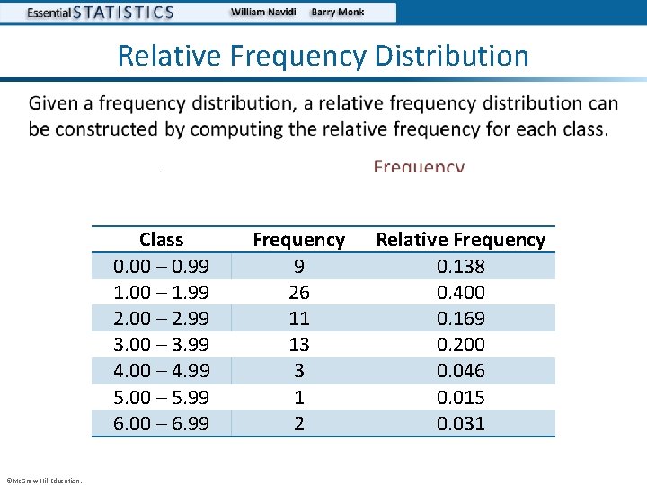
Relative Frequency Distribution • Class 0. 00 – 0. 99 1. 00 – 1. 99 2. 00 – 2. 99 3. 00 – 3. 99 4. 00 – 4. 99 5. 00 – 5. 99 6. 00 – 6. 99 ©Mc. Graw-Hill Education. Frequency 9 26 11 13 3 1 2 Relative Frequency 0. 138 0. 400 0. 169 0. 200 0. 046 0. 015 0. 031

Objective 2 Construct histograms ©Mc. Graw-Hill Education.

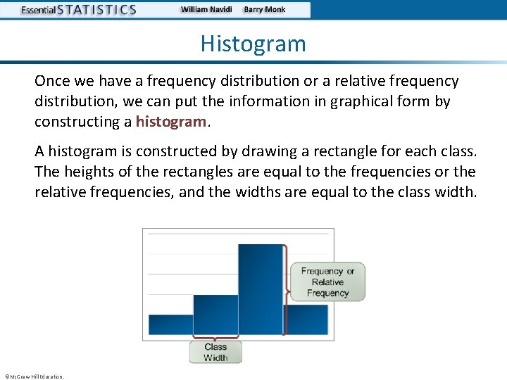
Histogram Once we have a frequency distribution or a relative frequency distribution, we can put the information in graphical form by constructing a histogram. A histogram is constructed by drawing a rectangle for each class. The heights of the rectangles are equal to the frequencies or the relative frequencies, and the widths are equal to the class width. ©Mc. Graw-Hill Education.

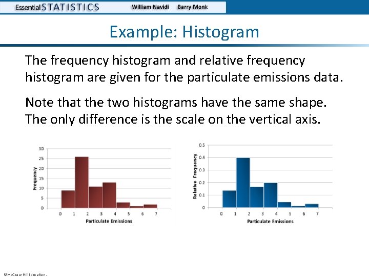
Example: Histogram The frequency histogram and relative frequency histogram are given for the particulate emissions data. Note that the two histograms have the same shape. The only difference is the scale on the vertical axis. ©Mc. Graw-Hill Education.

Choosing the Number of Classes There are no hard and fast rules for choosing the number of classes. In general, it is good to have more classes rather than fewer, but it is also good to have reasonably large frequencies in some of the classes. There are two principles that can guide the choice. • Too few classes produce a histogram lacking in detail. • Too many classes produce a histogram with too much detail, so that the main features of the data are obscured. ©Mc. Graw-Hill Education.

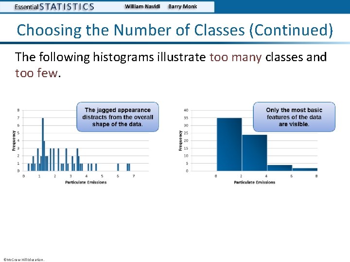
Choosing the Number of Classes (Continued) The following histograms illustrate too many classes and too few. ©Mc. Graw-Hill Education.

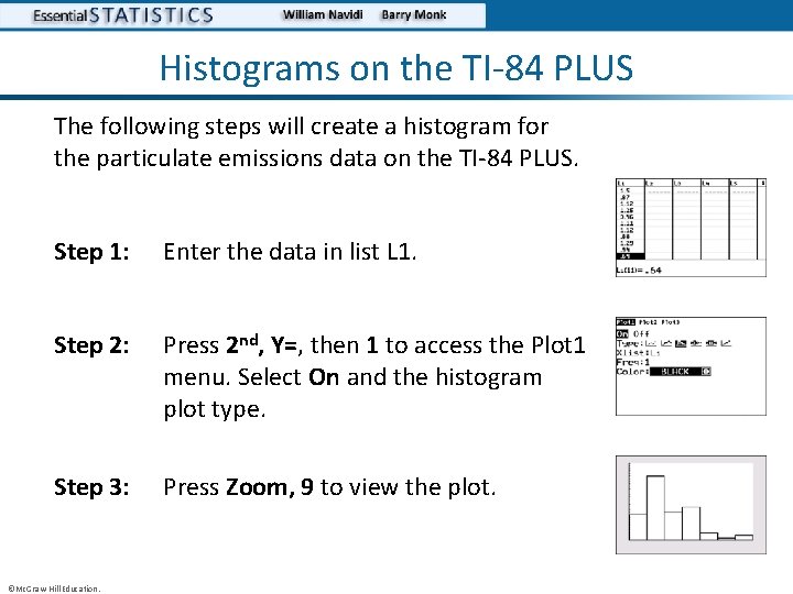
Histograms on the TI-84 PLUS The following steps will create a histogram for the particulate emissions data on the TI-84 PLUS. Step 1: Enter the data in list L 1. Step 2: Press 2 nd, Y=, then 1 to access the Plot 1 menu. Select On and the histogram plot type. Step 3: Press Zoom, 9 to view the plot. ©Mc. Graw-Hill Education.

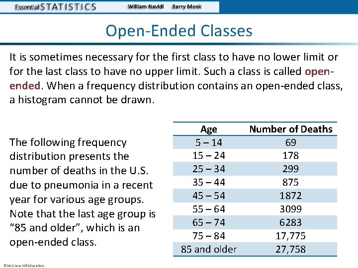
Open-Ended Classes It is sometimes necessary for the first class to have no lower limit or for the last class to have no upper limit. Such a class is called openended. When a frequency distribution contains an open-ended class, a histogram cannot be drawn. The following frequency distribution presents the number of deaths in the U. S. due to pneumonia in a recent year for various age groups. Note that the last age group is “ 85 and older”, which is an open-ended class. ©Mc. Graw-Hill Education. Age 5 – 14 15 – 24 25 – 34 35 – 44 45 – 54 55 – 64 65 – 74 75 – 84 85 and older Number of Deaths 69 178 299 875 1872 3099 6283 17, 775 27, 758

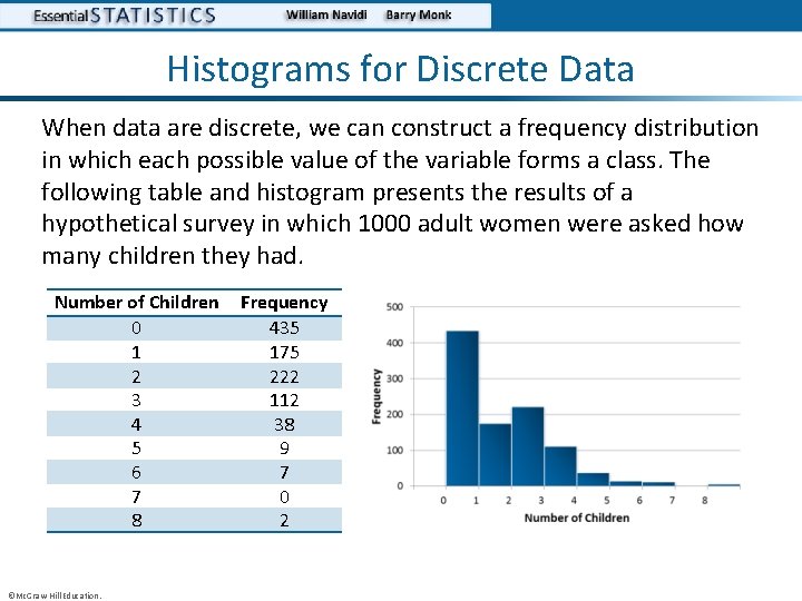
Histograms for Discrete Data When data are discrete, we can construct a frequency distribution in which each possible value of the variable forms a class. The following table and histogram presents the results of a hypothetical survey in which 1000 adult women were asked how many children they had. Number of Children 0 1 2 3 4 5 6 7 8 ©Mc. Graw-Hill Education. Frequency 435 175 222 112 38 9 7 0 2

Objective 3 Determine the shape of a distribution from a histogram ©Mc. Graw-Hill Education.

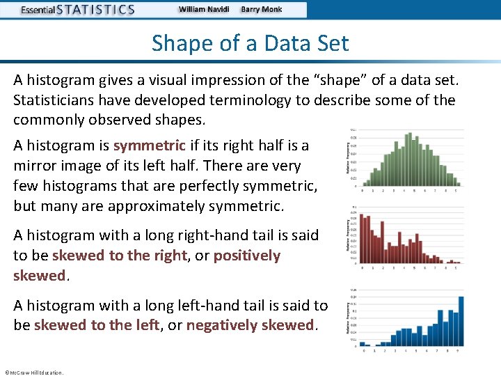
Shape of a Data Set A histogram gives a visual impression of the “shape” of a data set. Statisticians have developed terminology to describe some of the commonly observed shapes. A histogram is symmetric if its right half is a mirror image of its left half. There are very few histograms that are perfectly symmetric, but many are approximately symmetric. A histogram with a long right-hand tail is said to be skewed to the right, or positively skewed. A histogram with a long left-hand tail is said to be skewed to the left, or negatively skewed. ©Mc. Graw-Hill Education.

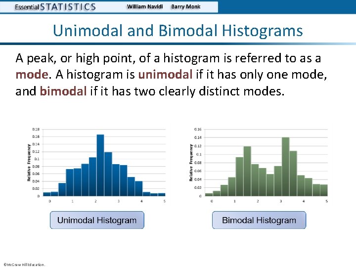
Unimodal and Bimodal Histograms A peak, or high point, of a histogram is referred to as a mode. A histogram is unimodal if it has only one mode, and bimodal if it has two clearly distinct modes. ©Mc. Graw-Hill Education.

You Should Know. . . • How to construct a frequency and relative frequency distribution for quantitative data • How to construct and interpret histograms • The guiding principles for choosing the number of classes in a histogram • How to construct a histogram on the TI-84 PLUS calculator • Some possible shapes of a data set including: – – – Symmetric Skewed to the right (positively skewed) Skewed to the left (negatively skewed) Unimodal Bimodal ©Mc. Graw-Hill Education.