Lecture Slides Elementary Statistics Tenth Edition and the

Lecture Slides Elementary Statistics Tenth Edition and the Triola Statistics Series by Mario F. Triola Slide 1

Chapter 11 Multinomial Experiments and Contingency Tables 11 -1 Overview 11 -2 Multinomial Experiments: Goodness-of-fit 11 -3 Contingency Tables: Independence and Homogeneity 11 -4 Mc. Nemar’s Test for Matched Pairs Copyright © 2007 Pearson Education, Inc Publishing as Pearson Addison-Wesley. Slide 2

Section 11 -1 & 11 -2 Overview and Multinomial Experiments: Goodness of Fit Created by Erin Hodgess, Houston, Texas Revised to accompany 10 th Edition, Jim Zimmer, Chattanooga State, Chattanooga, TN Slide 3

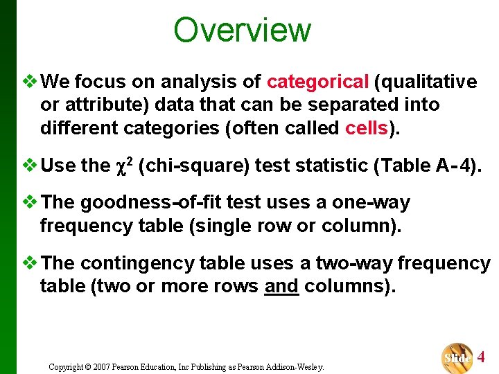
Overview v We focus on analysis of categorical (qualitative or attribute) data that can be separated into different categories (often called cells). v Use the 2 (chi-square) test statistic (Table A- 4). v The goodness-of-fit test uses a one-way frequency table (single row or column). v The contingency table uses a two-way frequency table (two or more rows and columns). Copyright © 2007 Pearson Education, Inc Publishing as Pearson Addison-Wesley. Slide 4

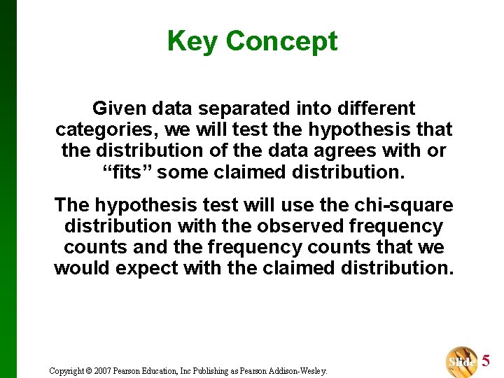
Key Concept Given data separated into different categories, we will test the hypothesis that the distribution of the data agrees with or “fits” some claimed distribution. The hypothesis test will use the chi-square distribution with the observed frequency counts and the frequency counts that we would expect with the claimed distribution. Copyright © 2007 Pearson Education, Inc Publishing as Pearson Addison-Wesley. Slide 5

Definition Multinomial Experiment This is an experiment that meets the following conditions: 1. The number of trials is fixed. 2. The trials are independent. 3. All outcomes of each trial must be classified into exactly one of several different categories. 4. The probabilities for the different categories remain constant for each trial. Copyright © 2007 Pearson Education, Inc Publishing as Pearson Addison-Wesley. Slide 6

Example: Last Digits of Weights When asked, people often provide weights that are somewhat lower than their actual weights. So how can researchers verify that weights were obtained through actual measurements instead of asking subjects? Copyright © 2007 Pearson Education, Inc Publishing as Pearson Addison-Wesley. Slide 7

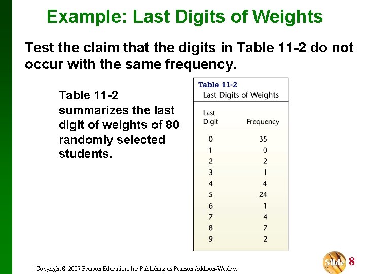
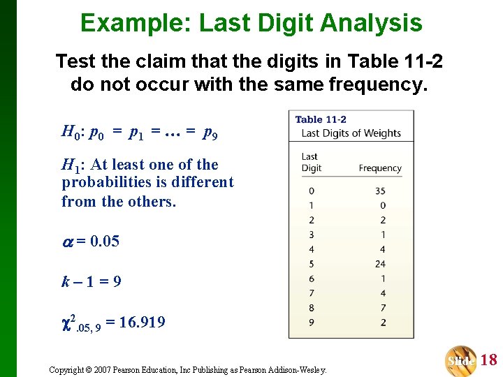
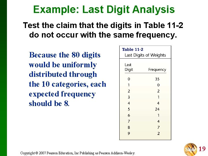
Example: Last Digits of Weights Test the claim that the digits in Table 11 -2 do not occur with the same frequency. Table 11 -2 summarizes the last digit of weights of 80 randomly selected students. Copyright © 2007 Pearson Education, Inc Publishing as Pearson Addison-Wesley. Slide 8

Example: Last Digits of Weights Verify that the four conditions of a multinomial experiment are satisfied. 1. The number of trials (last digits) is the fixed number 80. 2. The trials are independent, because the last digit of any individual’s weight does not affect the last digit of any other weight. 3. Each outcome (last digit) is classified into exactly 1 of 10 different categories. The categories are 0, 1, … , 9. 4. Finally, in testing the claim that the 10 digits are equally likely, each possible digit has a probability of 1/10, and by assumption, that probability remains constant for each subject. Copyright © 2007 Pearson Education, Inc Publishing as Pearson Addison-Wesley. Slide 9

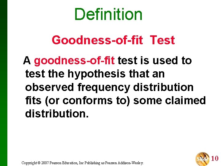
Definition Goodness-of-fit Test A goodness-of-fit test is used to test the hypothesis that an observed frequency distribution fits (or conforms to) some claimed distribution. Copyright © 2007 Pearson Education, Inc Publishing as Pearson Addison-Wesley. Slide 10

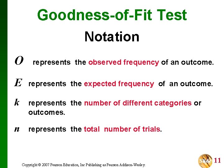
Goodness-of-Fit Test Notation O represents the observed frequency of an outcome. E represents the expected frequency of an outcome. k represents the number of different categories or outcomes. n represents the total number of trials. Copyright © 2007 Pearson Education, Inc Publishing as Pearson Addison-Wesley. Slide 11

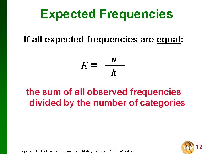
Expected Frequencies If all expected frequencies are equal: E= n k the sum of all observed frequencies divided by the number of categories Copyright © 2007 Pearson Education, Inc Publishing as Pearson Addison-Wesley. Slide 12

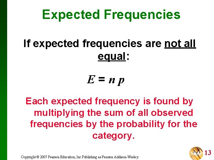
Expected Frequencies If expected frequencies are not all equal: E=np Each expected frequency is found by multiplying the sum of all observed frequencies by the probability for the category. Copyright © 2007 Pearson Education, Inc Publishing as Pearson Addison-Wesley. Slide 13

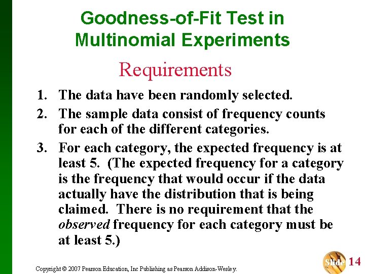
Goodness-of-Fit Test in Multinomial Experiments Requirements 1. The data have been randomly selected. 2. The sample data consist of frequency counts for each of the different categories. 3. For each category, the expected frequency is at least 5. (The expected frequency for a category is the frequency that would occur if the data actually have the distribution that is being claimed. There is no requirement that the observed frequency for each category must be at least 5. ) Copyright © 2007 Pearson Education, Inc Publishing as Pearson Addison-Wesley. Slide 14

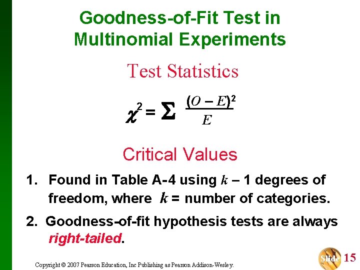
Goodness-of-Fit Test in Multinomial Experiments Test Statistics = 2 (O – E)2 E Critical Values 1. Found in Table A- 4 using k – 1 degrees of freedom, where k = number of categories. 2. Goodness-of-fit hypothesis tests are always right-tailed. Copyright © 2007 Pearson Education, Inc Publishing as Pearson Addison-Wesley. Slide 15

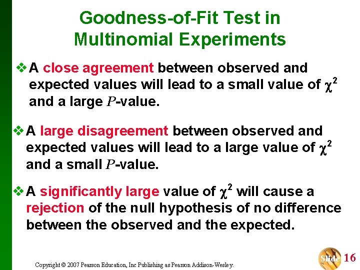
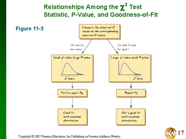
Goodness-of-Fit Test in Multinomial Experiments v A close agreement between observed and expected values will lead to a small value of 2 and a large P-value. v A large disagreement between observed and expected values will lead to a large value of 2 and a small P-value. v A significantly large value of 2 will cause a rejection of the null hypothesis of no difference between the observed and the expected. Copyright © 2007 Pearson Education, Inc Publishing as Pearson Addison-Wesley. Slide 16

Relationships Among the 2 Test Statistic, P-Value, and Goodness-of-Fit Figure 11 -3 Copyright © 2007 Pearson Education, Inc Publishing as Pearson Addison-Wesley. Slide 17

Example: Last Digit Analysis Test the claim that the digits in Table 11 -2 do not occur with the same frequency. H 0: p 0 = p 1 = = p 9 H 1: At least one of the probabilities is different from the others. = 0. 05 k– 1=9 2. 05, 9 = 16. 919 Copyright © 2007 Pearson Education, Inc Publishing as Pearson Addison-Wesley. Slide 18

Example: Last Digit Analysis Test the claim that the digits in Table 11 -2 do not occur with the same frequency. Because the 80 digits would be uniformly distributed through the 10 categories, each expected frequency should be 8. Copyright © 2007 Pearson Education, Inc Publishing as Pearson Addison-Wesley. Slide 19

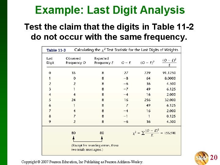
Example: Last Digit Analysis Test the claim that the digits in Table 11 -2 do not occur with the same frequency. Copyright © 2007 Pearson Education, Inc Publishing as Pearson Addison-Wesley. Slide 20

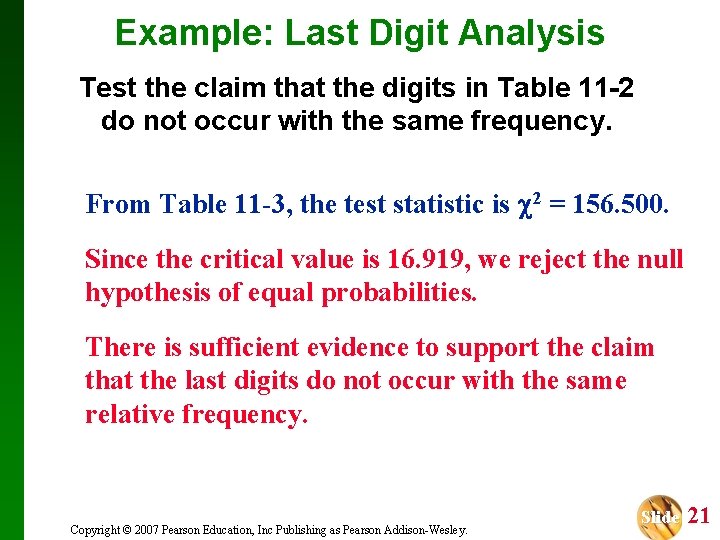
Example: Last Digit Analysis Test the claim that the digits in Table 11 -2 do not occur with the same frequency. From Table 11 -3, the test statistic is 2 = 156. 500. Since the critical value is 16. 919, we reject the null hypothesis of equal probabilities. There is sufficient evidence to support the claim that the last digits do not occur with the same relative frequency. Copyright © 2007 Pearson Education, Inc Publishing as Pearson Addison-Wesley. Slide 21

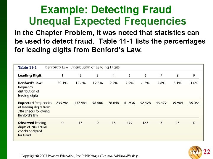
Example: Detecting Fraud Unequal Expected Frequencies In the Chapter Problem, it was noted that statistics can be used to detect fraud. Table 11 -1 lists the percentages for leading digits from Benford’s Law. Copyright © 2007 Pearson Education, Inc Publishing as Pearson Addison-Wesley. Slide 22

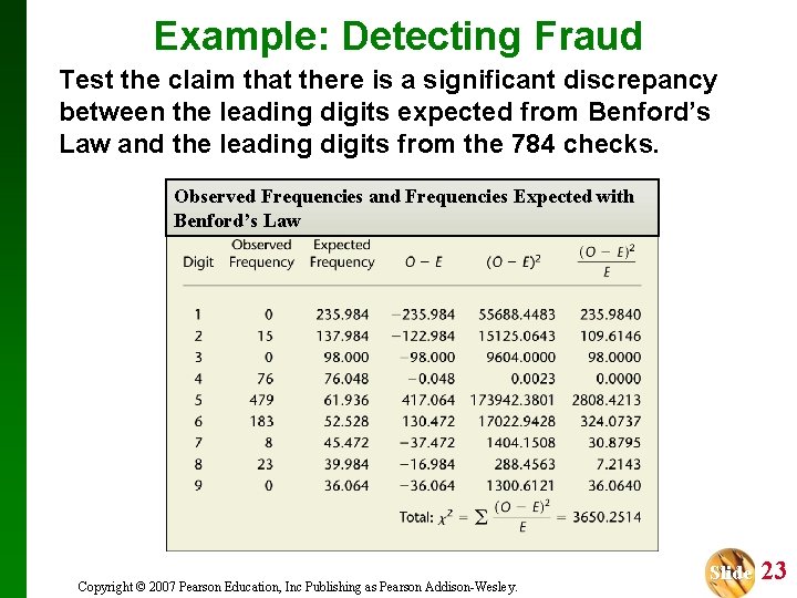
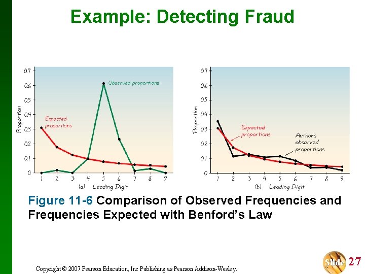
Example: Detecting Fraud Test the claim that there is a significant discrepancy between the leading digits expected from Benford’s Law and the leading digits from the 784 checks. Observed Frequencies and Frequencies Expected with Benford’s Law Copyright © 2007 Pearson Education, Inc Publishing as Pearson Addison-Wesley. Slide 23

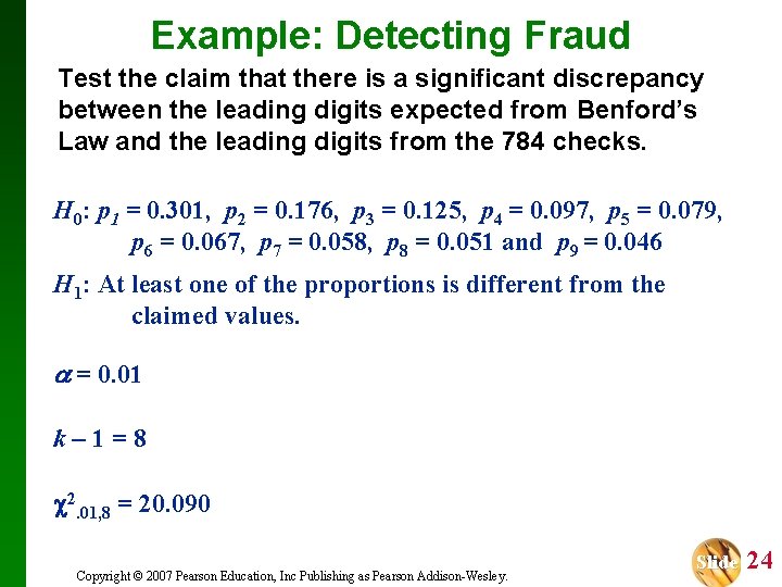
Example: Detecting Fraud Test the claim that there is a significant discrepancy between the leading digits expected from Benford’s Law and the leading digits from the 784 checks. H 0: p 1 = 0. 301, p 2 = 0. 176, p 3 = 0. 125, p 4 = 0. 097, p 5 = 0. 079, p 6 = 0. 067, p 7 = 0. 058, p 8 = 0. 051 and p 9 = 0. 046 H 1: At least one of the proportions is different from the claimed values. = 0. 01 k– 1=8 2. 01, 8 = 20. 090 Copyright © 2007 Pearson Education, Inc Publishing as Pearson Addison-Wesley. Slide 24

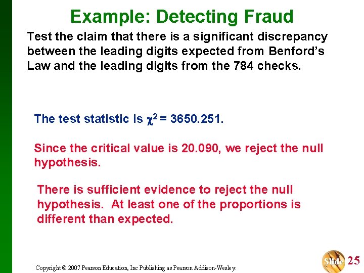
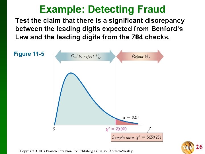
Example: Detecting Fraud Test the claim that there is a significant discrepancy between the leading digits expected from Benford’s Law and the leading digits from the 784 checks. The test statistic is 2 = 3650. 251. Since the critical value is 20. 090, we reject the null hypothesis. There is sufficient evidence to reject the null hypothesis. At least one of the proportions is different than expected. Copyright © 2007 Pearson Education, Inc Publishing as Pearson Addison-Wesley. Slide 25

Example: Detecting Fraud Test the claim that there is a significant discrepancy between the leading digits expected from Benford’s Law and the leading digits from the 784 checks. Figure 11 -5 Copyright © 2007 Pearson Education, Inc Publishing as Pearson Addison-Wesley. Slide 26

Example: Detecting Fraud Figure 11 -6 Comparison of Observed Frequencies and Frequencies Expected with Benford’s Law Copyright © 2007 Pearson Education, Inc Publishing as Pearson Addison-Wesley. Slide 27

Recap In this section we have discussed: Multinomial Experiments: Goodness-of-Fit - Equal Expected Frequencies - Unequal Expected Frequencies Test the hypothesis that an observed frequency distribution fits (or conforms to) some claimed distribution. Copyright © 2007 Pearson Education, Inc Publishing as Pearson Addison-Wesley. Slide 28

Section 11 -3 Contingency Tables: Independence and Homogeneity Created by Erin Hodgess, Houston, Texas Revised to accompany 10 th Edition, Jim Zimmer, Chattanooga State, Chattanooga, TN Slide 29

Key Concept In this section we consider contingency tables (or two-way frequency tables), which include frequency counts for categorical data arranged in a table with a least two rows and at least two columns. We present a method for testing the claim that the row and column variables are independent of each other. We will use the same method for a test of homogeneity, whereby we test the claim that different populations have the same proportion of some characteristics. Copyright © 2007 Pearson Education, Inc Publishing as Pearson Addison-Wesley. Slide 30

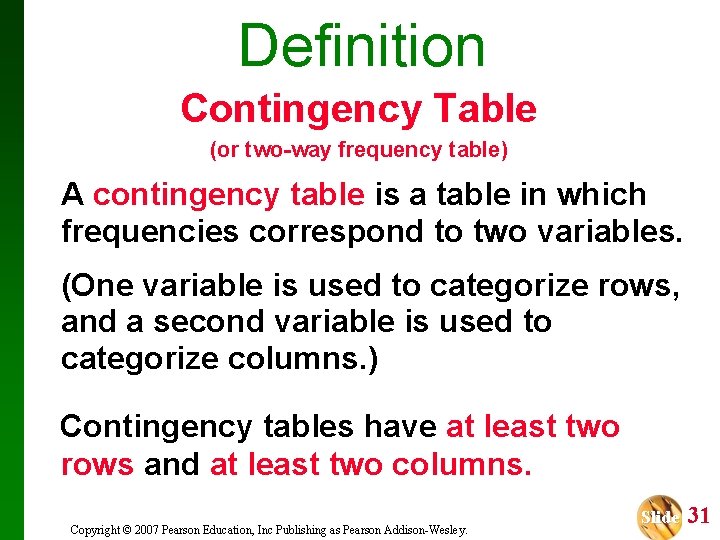
Definition Contingency Table (or two-way frequency table) A contingency table is a table in which frequencies correspond to two variables. (One variable is used to categorize rows, and a second variable is used to categorize columns. ) Contingency tables have at least two rows and at least two columns. Copyright © 2007 Pearson Education, Inc Publishing as Pearson Addison-Wesley. Slide 31

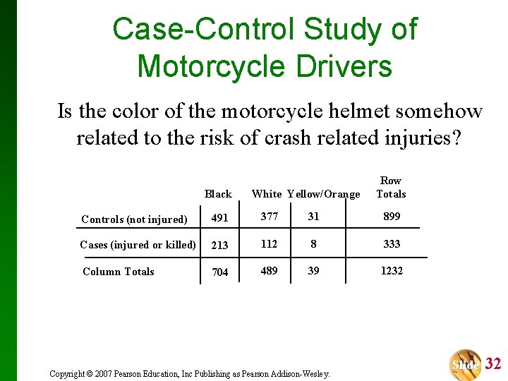
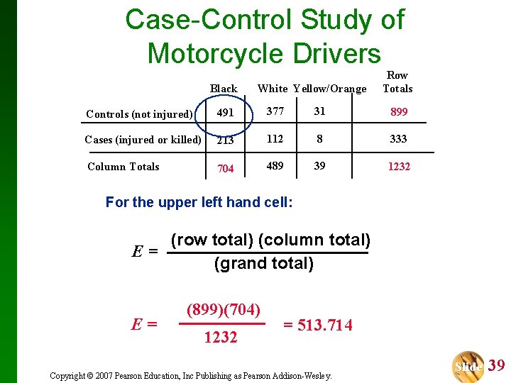
Case-Control Study of Motorcycle Drivers Is the color of the motorcycle helmet somehow related to the risk of crash related injuries? Black White Yellow/Orange Row Totals Controls (not injured) 491 377 31 899 Cases (injured or killed) 213 112 8 333 Column Totals 704 489 39 1232 Copyright © 2007 Pearson Education, Inc Publishing as Pearson Addison-Wesley. Slide 32

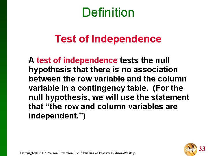
Definition Test of Independence A test of independence tests the null hypothesis that there is no association between the row variable and the column variable in a contingency table. (For the null hypothesis, we will use the statement that “the row and column variables are independent. ”) Copyright © 2007 Pearson Education, Inc Publishing as Pearson Addison-Wesley. Slide 33

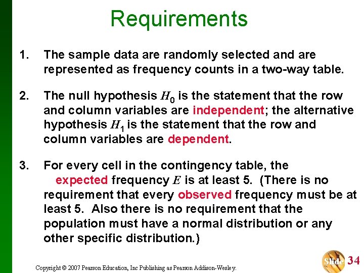
Requirements 1. The sample data are randomly selected and are represented as frequency counts in a two-way table. 2. The null hypothesis H 0 is the statement that the row and column variables are independent; the alternative hypothesis H 1 is the statement that the row and column variables are dependent. 3. For every cell in the contingency table, the expected frequency E is at least 5. (There is no requirement that every observed frequency must be at least 5. Also there is no requirement that the population must have a normal distribution or any other specific distribution. ) Copyright © 2007 Pearson Education, Inc Publishing as Pearson Addison-Wesley. Slide 34

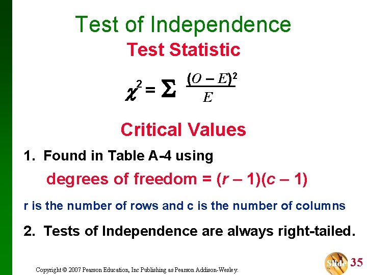
Test of Independence Test Statistic = 2 (O – E)2 E Critical Values 1. Found in Table A-4 using degrees of freedom = (r – 1)(c – 1) r is the number of rows and c is the number of columns 2. Tests of Independence are always right-tailed. Copyright © 2007 Pearson Education, Inc Publishing as Pearson Addison-Wesley. Slide 35

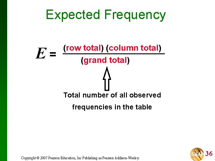
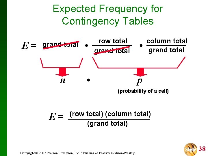
Expected Frequency E= (row total) (column total) (grand total) Total number of all observed frequencies in the table Copyright © 2007 Pearson Education, Inc Publishing as Pearson Addison-Wesley. Slide 36

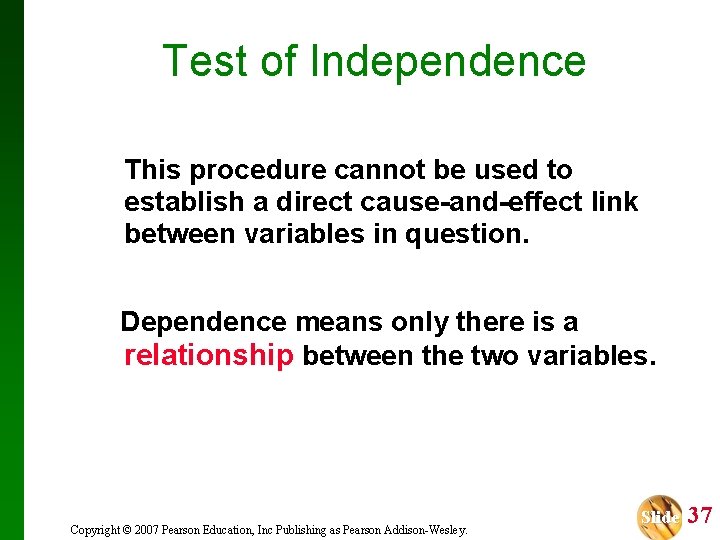
Test of Independence This procedure cannot be used to establish a direct cause-and-effect link between variables in question. Dependence means only there is a relationship between the two variables. Copyright © 2007 Pearson Education, Inc Publishing as Pearson Addison-Wesley. Slide 37

Expected Frequency for Contingency Tables E= grand total n • row total grand total • • column total grand total p (probability of a cell) E= (row total) (column total) (grand total) Copyright © 2007 Pearson Education, Inc Publishing as Pearson Addison-Wesley. Slide 38

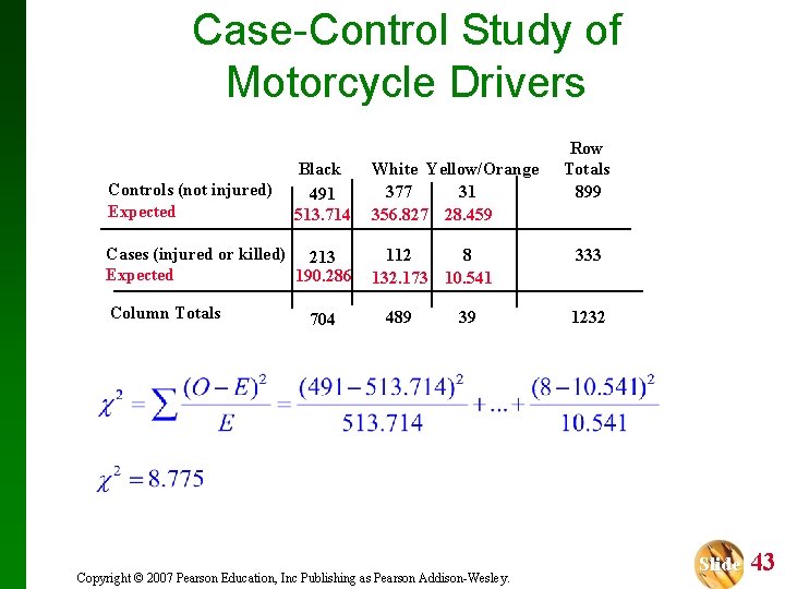
Case-Control Study of Motorcycle Drivers Black White Yellow/Orange Row Totals Controls (not injured) 491 377 31 899 Cases (injured or killed) 213 112 8 333 Column Totals 704 489 39 1232 For the upper left hand cell: (row total) (column total) E= (grand total) E= (899)(704) 1232 = 513. 714 Copyright © 2007 Pearson Education, Inc Publishing as Pearson Addison-Wesley. Slide 39

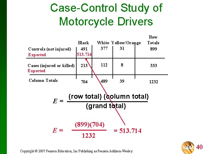
Case-Control Study of Motorcycle Drivers Black 491 513. 714 Controls (not injured) Expected White Yellow/Orange 377 31 Row Totals 899 Cases (injured or killed) Expected 213 112 8 333 Column Totals 704 489 39 1232 (row total) (column total) E= (grand total) E= (899)(704) 1232 = 513. 714 Copyright © 2007 Pearson Education, Inc Publishing as Pearson Addison-Wesley. Slide 40

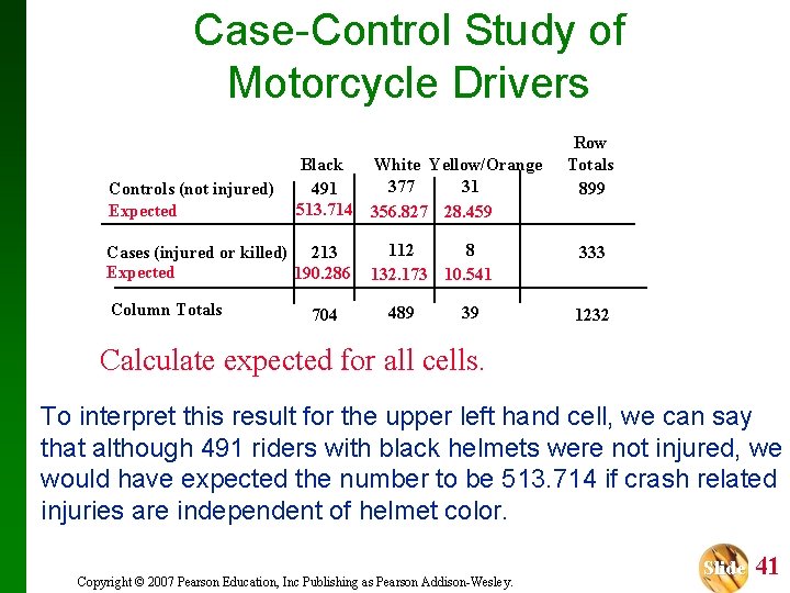
Case-Control Study of Motorcycle Drivers Controls (not injured) Expected Black 491 513. 714 Cases (injured or killed) 213 Expected 190. 286 Column Totals 704 White Yellow/Orange 377 31 356. 827 28. 459 112 8 132. 173 10. 541 489 39 Row Totals 899 333 1232 Calculate expected for all cells. To interpret this result for the upper left hand cell, we can say that although 491 riders with black helmets were not injured, we would have expected the number to be 513. 714 if crash related injuries are independent of helmet color. Copyright © 2007 Pearson Education, Inc Publishing as Pearson Addison-Wesley. Slide 41

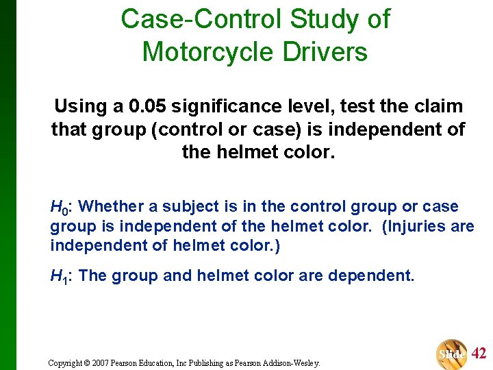
Case-Control Study of Motorcycle Drivers Using a 0. 05 significance level, test the claim that group (control or case) is independent of the helmet color. H 0: Whether a subject is in the control group or case group is independent of the helmet color. (Injuries are independent of helmet color. ) H 1: The group and helmet color are dependent. Copyright © 2007 Pearson Education, Inc Publishing as Pearson Addison-Wesley. Slide 42

Case-Control Study of Motorcycle Drivers Controls (not injured) Expected Black 491 513. 714 Cases (injured or killed) 213 Expected 190. 286 Column Totals 704 White Yellow/Orange 377 31 356. 827 28. 459 112 8 132. 173 10. 541 489 39 Copyright © 2007 Pearson Education, Inc Publishing as Pearson Addison-Wesley. Row Totals 899 333 1232 Slide 43

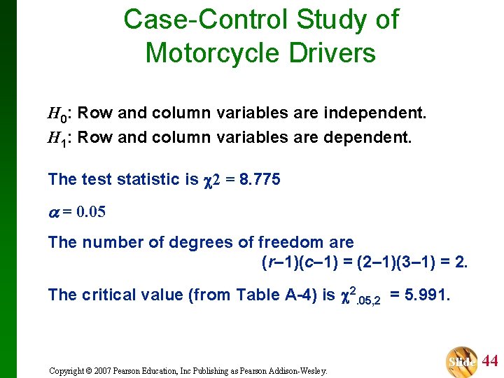
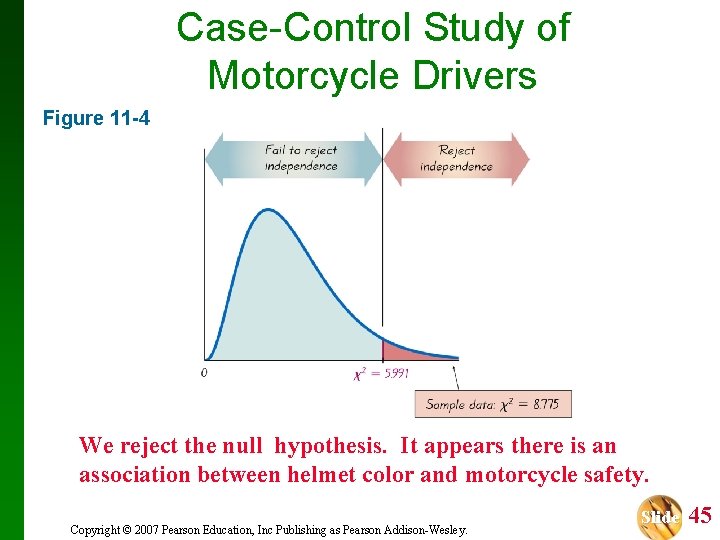
Case-Control Study of Motorcycle Drivers H 0: Row and column variables are independent. H 1: Row and column variables are dependent. The test statistic is 2 = 8. 775 = 0. 05 The number of degrees of freedom are (r– 1)(c– 1) = (2– 1)(3– 1) = 2. The critical value (from Table A-4) is 2. 05, 2 = 5. 991. Copyright © 2007 Pearson Education, Inc Publishing as Pearson Addison-Wesley. Slide 44

Case-Control Study of Motorcycle Drivers Figure 11 -4 We reject the null hypothesis. It appears there is an association between helmet color and motorcycle safety. Copyright © 2007 Pearson Education, Inc Publishing as Pearson Addison-Wesley. Slide 45

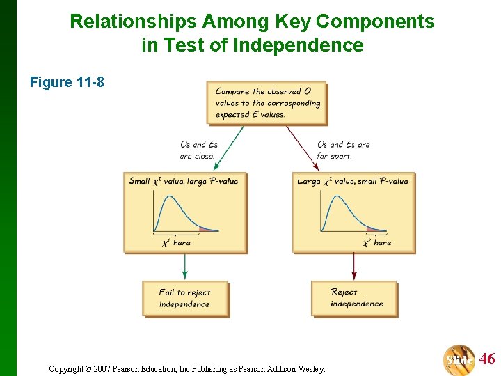
Relationships Among Key Components in Test of Independence Figure 11 -8 Copyright © 2007 Pearson Education, Inc Publishing as Pearson Addison-Wesley. Slide 46

Definition Test of Homogeneity In a test of homogeneity, we test the claim that different populations have the same proportions of some characteristics. Copyright © 2007 Pearson Education, Inc Publishing as Pearson Addison-Wesley. Slide 47

How to Distinguish Between a Test of Homogeneity and a Test for Independence: Were predetermined sample sizes used for different populations (test of homogeneity), or was one big sample drawn so both row and column totals were determined randomly (test of independence)? Copyright © 2007 Pearson Education, Inc Publishing as Pearson Addison-Wesley. Slide 48

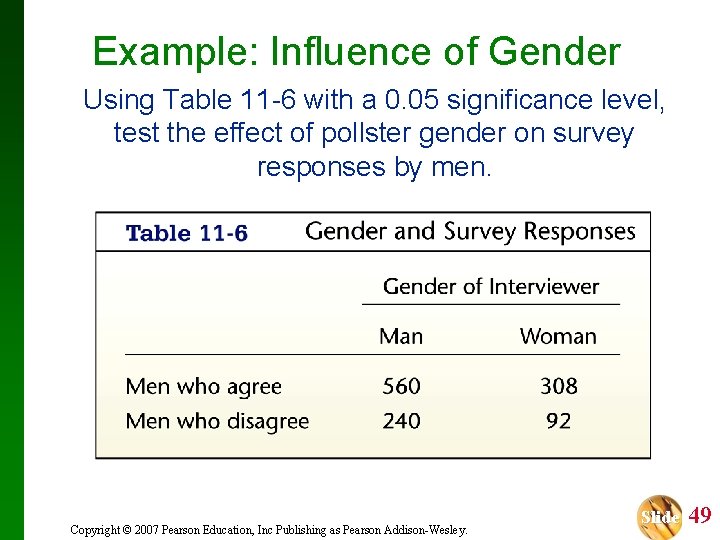
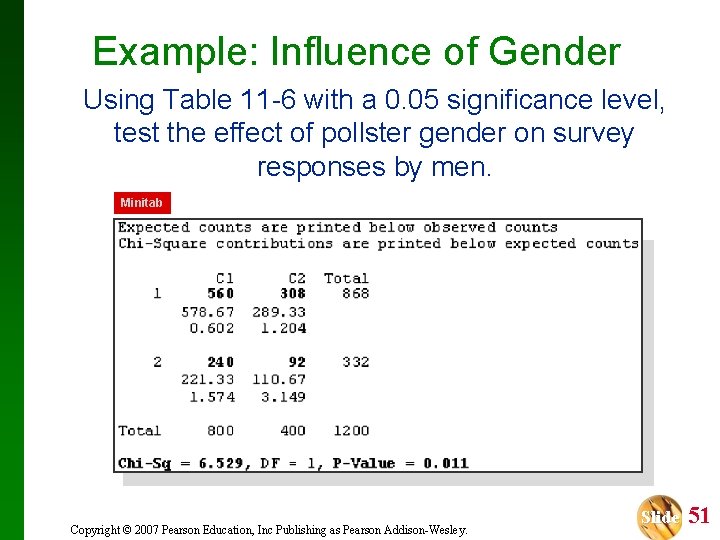
Example: Influence of Gender Using Table 11 -6 with a 0. 05 significance level, test the effect of pollster gender on survey responses by men. Copyright © 2007 Pearson Education, Inc Publishing as Pearson Addison-Wesley. Slide 49

Example: Influence of Gender Using Table 11 -6 with a 0. 05 significance level, test the effect of pollster gender on survey responses by men. H 0: The proportions of agree/disagree responses are the same for the subjects interviewed by men and the subjects interviewed by women. H 1: The proportions are different. Copyright © 2007 Pearson Education, Inc Publishing as Pearson Addison-Wesley. Slide 50

Example: Influence of Gender Using Table 11 -6 with a 0. 05 significance level, test the effect of pollster gender on survey responses by men. Minitab Copyright © 2007 Pearson Education, Inc Publishing as Pearson Addison-Wesley. Slide 51

Recap In this section we have discussed: Contingency tables where categorical data is arranged in a table with a least two rows and at least two columns. * Test of Independence tests the claim that the row and column variables are independent of each other. * Test of Homogeneity tests the claim that different populations have the same proportion of some characteristics. Copyright © 2007 Pearson Education, Inc Publishing as Pearson Addison-Wesley. Slide 52

Section 11 -4 Mc. Nemar’s Test for Matched Pairs Created by Erin Hodgess, Houston, Texas Revised to accompany 10 th Edition, Jim Zimmer, Chattanooga State, Chattanooga, TN Slide 53

Key Concept The Contingency table procedures in Section 11 -3 are based on independent data. For 2 x 2 tables consisting of frequency counts that result from matched pairs, we do not have independence, and for such cases, we can use Mc. Nemar’s test for matched pairs. Copyright © 2007 Pearson Education, Inc Publishing as Pearson Addison-Wesley. Slide 54

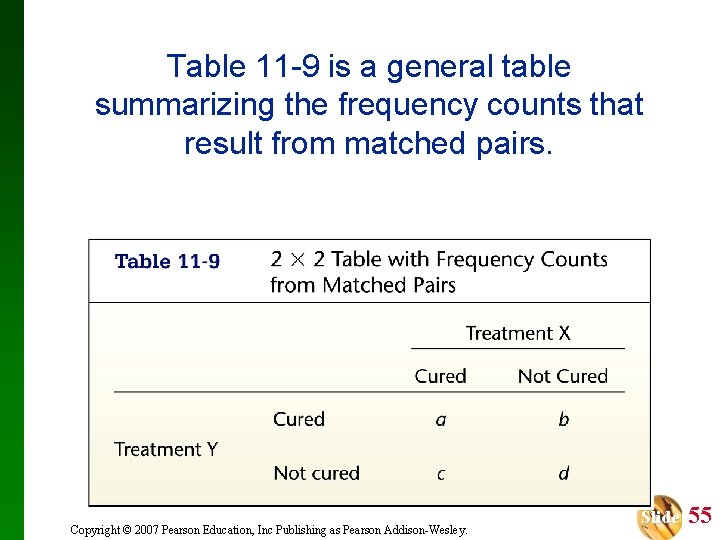
Table 11 -9 is a general table summarizing the frequency counts that result from matched pairs. Copyright © 2007 Pearson Education, Inc Publishing as Pearson Addison-Wesley. Slide 55

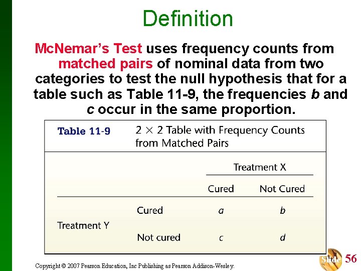
Definition Mc. Nemar’s Test uses frequency counts from matched pairs of nominal data from two categories to test the null hypothesis that for a table such as Table 11 -9, the frequencies b and c occur in the same proportion. Copyright © 2007 Pearson Education, Inc Publishing as Pearson Addison-Wesley. Slide 56

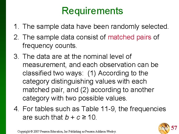
Requirements 1. The sample data have been randomly selected. 2. The sample data consist of matched pairs of frequency counts. 3. The data are at the nominal level of measurement, and each observation can be classified two ways: (1) According to the category distinguishing values with each matched pair, and (2) according to another category with two possible values. 4. For tables such as Table 11 -9, the frequencies are such that b + c ≥ 10. Copyright © 2007 Pearson Education, Inc Publishing as Pearson Addison-Wesley. Slide 57

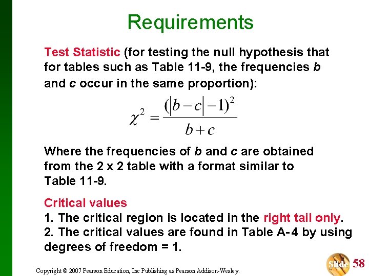
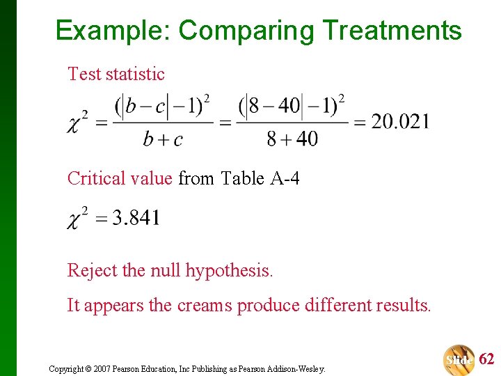
Requirements Test Statistic (for testing the null hypothesis that for tables such as Table 11 -9, the frequencies b and c occur in the same proportion): Where the frequencies of b and c are obtained from the 2 x 2 table with a format similar to Table 11 -9. Critical values 1. The critical region is located in the right tail only. 2. The critical values are found in Table A- 4 by using degrees of freedom = 1. Slide 58 Copyright © 2007 Pearson Education, Inc Publishing as Pearson Addison-Wesley.

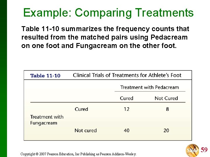
Example: Comparing Treatments Table 11 -10 summarizes the frequency counts that resulted from the matched pairs using Pedacream on one foot and Fungacream on the other foot. Copyright © 2007 Pearson Education, Inc Publishing as Pearson Addison-Wesley. Slide 59

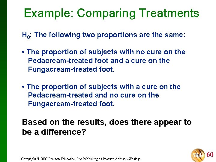
Example: Comparing Treatments H 0: The following two proportions are the same: • The proportion of subjects with no cure on the Pedacream-treated foot and a cure on the Fungacream-treated foot. • The proportion of subjects with a cure on the Pedacream-treated and no cure on the Fungacream-treated foot. Based on the results, does there appear to be a difference? Copyright © 2007 Pearson Education, Inc Publishing as Pearson Addison-Wesley. Slide 60

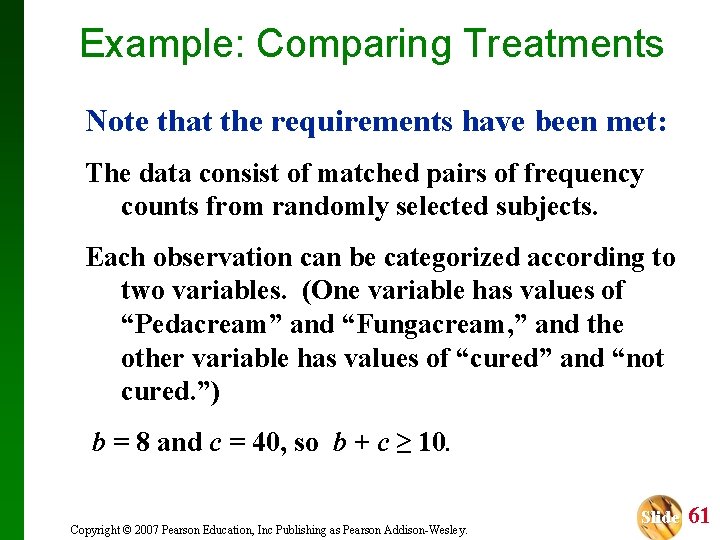
Example: Comparing Treatments Note that the requirements have been met: The data consist of matched pairs of frequency counts from randomly selected subjects. Each observation can be categorized according to two variables. (One variable has values of “Pedacream” and “Fungacream, ” and the other variable has values of “cured” and “not cured. ”) b = 8 and c = 40, so b + c ≥ 10. Copyright © 2007 Pearson Education, Inc Publishing as Pearson Addison-Wesley. Slide 61

Example: Comparing Treatments Test statistic Critical value from Table A-4 Reject the null hypothesis. It appears the creams produce different results. Copyright © 2007 Pearson Education, Inc Publishing as Pearson Addison-Wesley. Slide 62

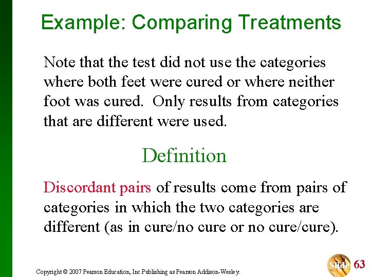
Example: Comparing Treatments Note that the test did not use the categories where both feet were cured or where neither foot was cured. Only results from categories that are different were used. Definition . Discordant pairs of results come from pairs of categories in which the two categories are different (as in cure/no cure or no cure/cure). Copyright © 2007 Pearson Education, Inc Publishing as Pearson Addison-Wesley. Slide 63

Recap In this section we have discussed: Mc. Nemar’s test for matched pairs. • Data are place in a 2 x 2 table where each observation is classified in two ways. • The test only compares categories that are different (discordant pairs). Copyright © 2007 Pearson Education, Inc Publishing as Pearson Addison-Wesley. Slide 64