Elementary Statistics Thirteenth Edition Chapter 2 Summarizing and

Elementary Statistics Thirteenth Edition Chapter 2 Summarizing and Graphing Data Copyright © 2018, 2014, 2012 Pearson Education, Inc. All Rights Reserved

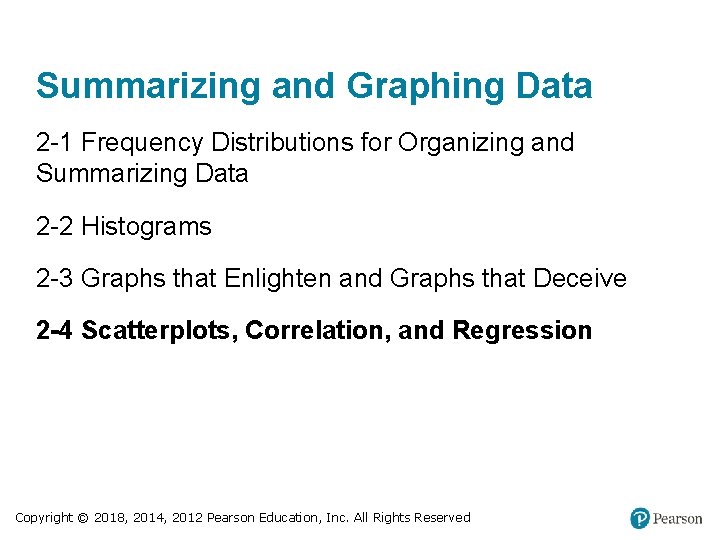
Summarizing and Graphing Data 2 -1 Frequency Distributions for Organizing and Summarizing Data 2 -2 Histograms 2 -3 Graphs that Enlighten and Graphs that Deceive 2 -4 Scatterplots, Correlation, and Regression Copyright © 2018, 2014, 2012 Pearson Education, Inc. All Rights Reserved

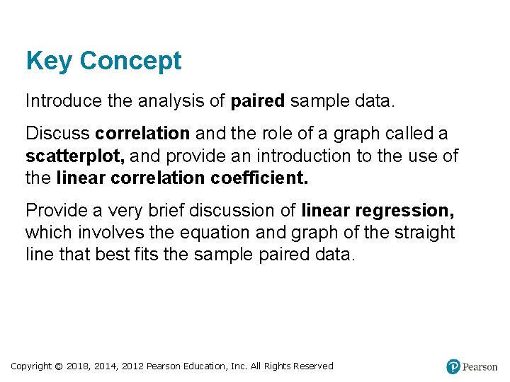
Key Concept Introduce the analysis of paired sample data. Discuss correlation and the role of a graph called a scatterplot, and provide an introduction to the use of the linear correlation coefficient. Provide a very brief discussion of linear regression, which involves the equation and graph of the straight line that best fits the sample paired data. Copyright © 2018, 2014, 2012 Pearson Education, Inc. All Rights Reserved

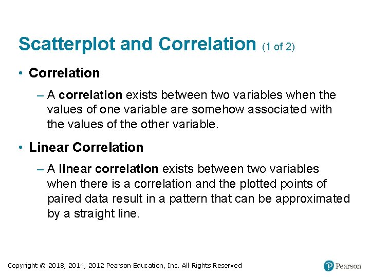
Scatterplot and Correlation (1 of 2) • Correlation – A correlation exists between two variables when the values of one variable are somehow associated with the values of the other variable. • Linear Correlation – A linear correlation exists between two variables when there is a correlation and the plotted points of paired data result in a pattern that can be approximated by a straight line. Copyright © 2018, 2014, 2012 Pearson Education, Inc. All Rights Reserved

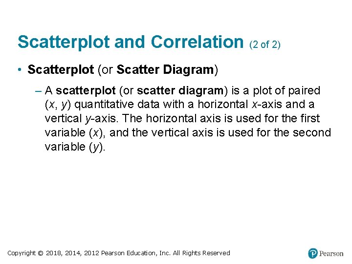
Scatterplot and Correlation (2 of 2) • Scatterplot (or Scatter Diagram) – A scatterplot (or scatter diagram) is a plot of paired (x, y) quantitative data with a horizontal x-axis and a vertical y-axis. The horizontal axis is used for the first variable (x), and the vertical axis is used for the second variable (y). Copyright © 2018, 2014, 2012 Pearson Education, Inc. All Rights Reserved

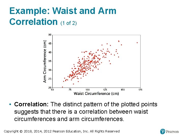
Example: Waist and Arm Correlation (1 of 2) • Correlation: The distinct pattern of the plotted points suggests that there is a correlation between waist circumferences and arm circumferences. Copyright © 2018, 2014, 2012 Pearson Education, Inc. All Rights Reserved

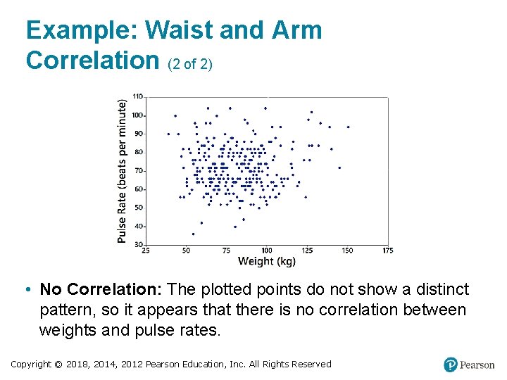
Example: Waist and Arm Correlation (2 of 2) • No Correlation: The plotted points do not show a distinct pattern, so it appears that there is no correlation between weights and pulse rates. Copyright © 2018, 2014, 2012 Pearson Education, Inc. All Rights Reserved

Linear Correlation Coefficient r • Linear Correlation Coefficient r – The linear correlation coefficient is denoted by r, and it measures the strength of the linear association between two variables. Copyright © 2018, 2014, 2012 Pearson Education, Inc. All Rights Reserved

Using r for Determining Correlation The computed value of the linear correlation coefficient, r, is always between − 1 and 1. • If r is close to − 1 or close to 1, there appears to be a correlation. • If r is close to 0, there does not appear to be a linear correlation. Copyright © 2018, 2014, 2012 Pearson Education, Inc. All Rights Reserved

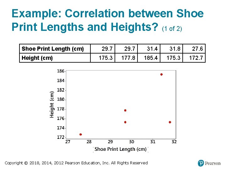
Example: Correlation between Shoe Print Lengths and Heights? (1 of 2) Shoe Print Length (cm) Height (cm) 29. 7 31. 4 31. 8 27. 6 175. 3 177. 8 185. 4 175. 3 172. 7 Copyright © 2018, 2014, 2012 Pearson Education, Inc. All Rights Reserved

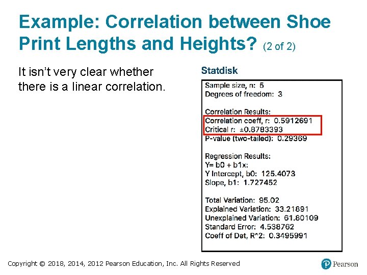
Example: Correlation between Shoe Print Lengths and Heights? (2 of 2) It isn’t very clear whethere is a linear correlation. Copyright © 2018, 2014, 2012 Pearson Education, Inc. All Rights Reserved

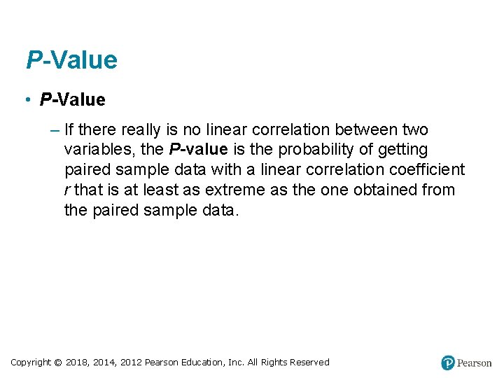
P-Value • P-Value – If there really is no linear correlation between two variables, the P-value is the probability of getting paired sample data with a linear correlation coefficient r that is at least as extreme as the one obtained from the paired sample data. Copyright © 2018, 2014, 2012 Pearson Education, Inc. All Rights Reserved

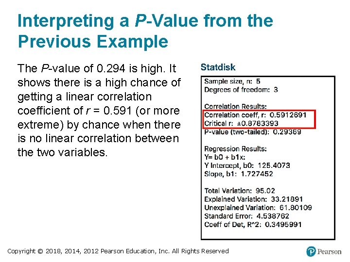
Interpreting a P-Value from the Previous Example The P-value of 0. 294 is high. It shows there is a high chance of getting a linear correlation coefficient of r = 0. 591 (or more extreme) by chance when there is no linear correlation between the two variables. Copyright © 2018, 2014, 2012 Pearson Education, Inc. All Rights Reserved

Interpreting a P-Value from the Example Where n = 5 Because the likelihood of getting r = 0. 591 or a more extreme value is so high (29. 4% chance), we conclude there is not sufficient evidence to conclude there is a linear correlation between shoe print lengths and heights. Copyright © 2018, 2014, 2012 Pearson Education, Inc. All Rights Reserved

Interpreting a P-Value Only a small P-value, such as 0. 05 or less (or a 5% chance or less), suggests that the sample results are not likely to occur by chance when there is no linear correlation, so a small P-value supports a conclusion that there is a linear correlation between the two variables. Copyright © 2018, 2014, 2012 Pearson Education, Inc. All Rights Reserved

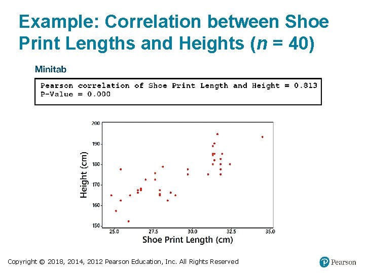
Example: Correlation between Shoe Print Lengths and Heights (n = 40) Copyright © 2018, 2014, 2012 Pearson Education, Inc. All Rights Reserved

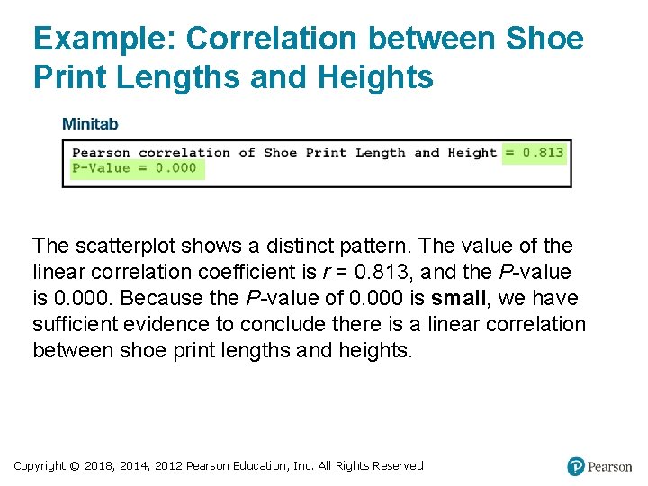
Example: Correlation between Shoe Print Lengths and Heights The scatterplot shows a distinct pattern. The value of the linear correlation coefficient is r = 0. 813, and the P-value is 0. 000. Because the P-value of 0. 000 is small, we have sufficient evidence to conclude there is a linear correlation between shoe print lengths and heights. Copyright © 2018, 2014, 2012 Pearson Education, Inc. All Rights Reserved

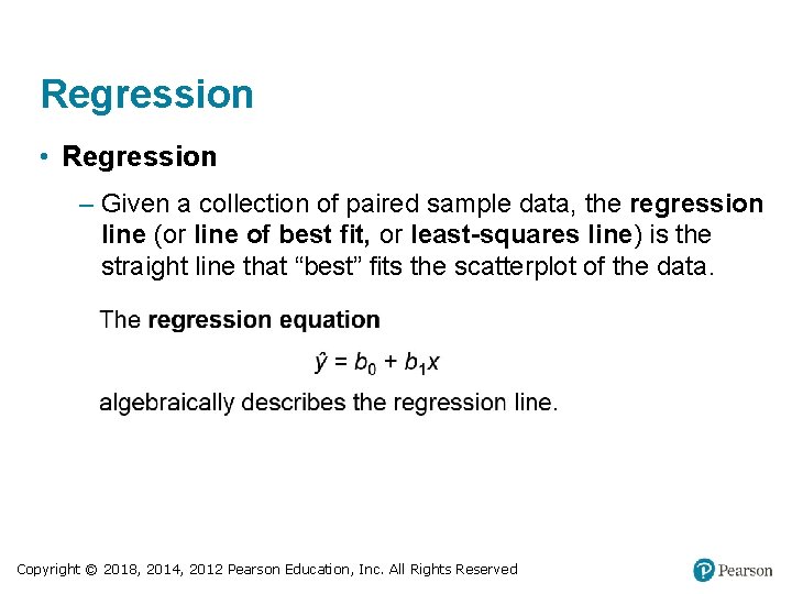
Regression • Regression – Given a collection of paired sample data, the regression line (or line of best fit, or least-squares line) is the straight line that “best” fits the scatterplot of the data. Copyright © 2018, 2014, 2012 Pearson Education, Inc. All Rights Reserved

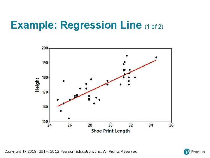
Example: Regression Line (1 of 2) Copyright © 2018, 2014, 2012 Pearson Education, Inc. All Rights Reserved

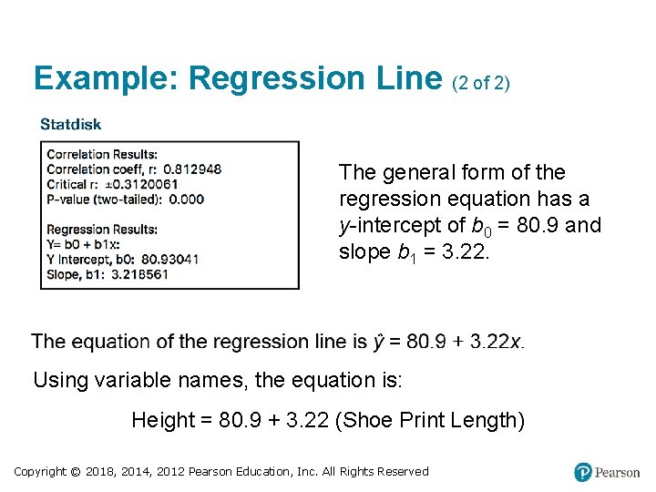
Example: Regression Line (2 of 2) The general form of the regression equation has a y-intercept of b 0 = 80. 9 and slope b 1 = 3. 22. Using variable names, the equation is: Height = 80. 9 + 3. 22 (Shoe Print Length) Copyright © 2018, 2014, 2012 Pearson Education, Inc. All Rights Reserved