Elementary Statistics Thirteenth Edition Chapter 13 Nonparametric Tests

Elementary Statistics Thirteenth Edition Chapter 13 Nonparametric Tests Copyright © 2018, 2014, 2012 Pearson Education, Inc. All Rights Reserved

Nonparametric Tests 13 -1 Basics of Nonparametric Tests 13 -2 Sign Test 13 -3 Wilcoxon Signed-Ranks Test for Matched Pairs 13 -4 Wilcoxon Rank-Sum Test for Two Independent Samples 13 -5 Kruskal-Wallis Test for Three or More Samples 13 -6 Rank Correlation 13 -7 Runs Test for Randomness Copyright © 2018, 2014, 2012 Pearson Education, Inc. All Rights Reserved

Key Concept This section describes the Kruskal-Wallis test, which uses ranks of data from three or more independent simple random samples to test the null hypothesis that the samples come from populations with the same median. Copyright © 2018, 2014, 2012 Pearson Education, Inc. All Rights Reserved

Kruskal-Wallis test • Kruskal-Wallis test – The Kruskal-Wallis test (also called the H test) is a nonparametric test that uses ranks of combined simple random samples from three or more independent populations to test the null hypothesis that the populations have the same median. Copyright © 2018, 2014, 2012 Pearson Education, Inc. All Rights Reserved

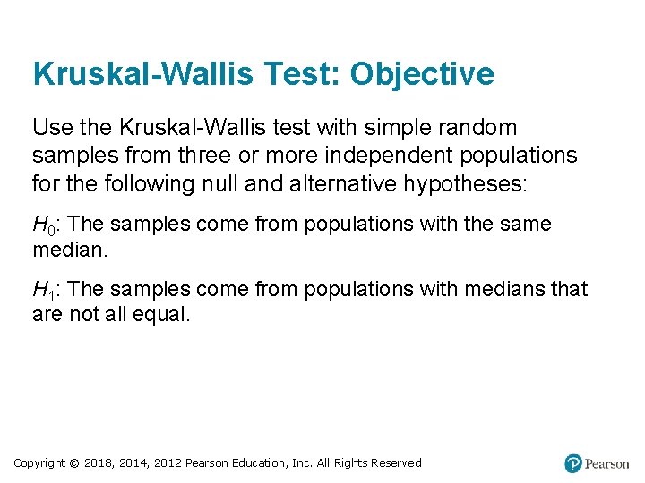
Kruskal-Wallis Test: Objective Use the Kruskal-Wallis test with simple random samples from three or more independent populations for the following null and alternative hypotheses: H 0: The samples come from populations with the same median. H 1: The samples come from populations with medians that are not all equal. Copyright © 2018, 2014, 2012 Pearson Education, Inc. All Rights Reserved

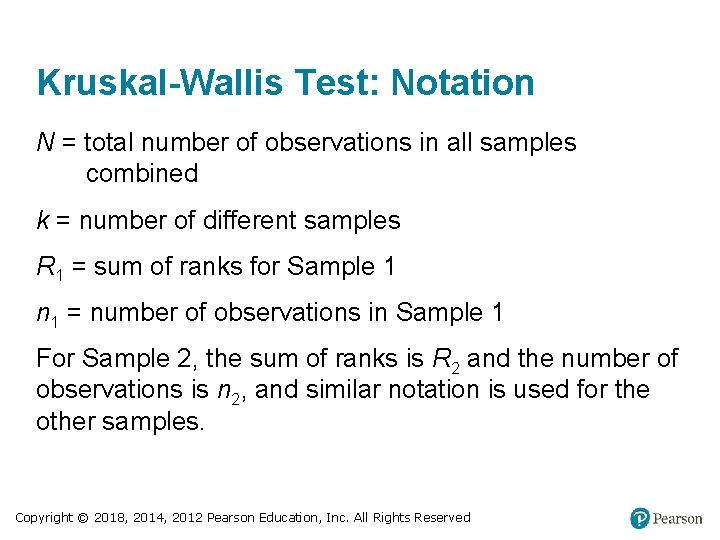
Kruskal-Wallis Test: Notation N = total number of observations in all samples combined k = number of different samples R 1 = sum of ranks for Sample 1 n 1 = number of observations in Sample 1 For Sample 2, the sum of ranks is R 2 and the number of observations is n 2, and similar notation is used for the other samples. Copyright © 2018, 2014, 2012 Pearson Education, Inc. All Rights Reserved

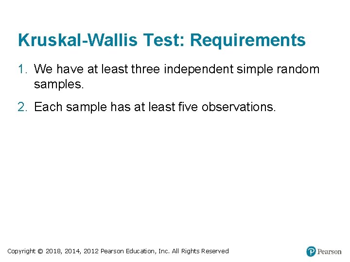
Kruskal-Wallis Test: Requirements 1. We have at least three independent simple random samples. 2. Each sample has at least five observations. Copyright © 2018, 2014, 2012 Pearson Education, Inc. All Rights Reserved

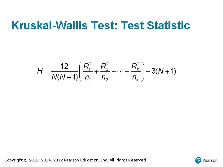
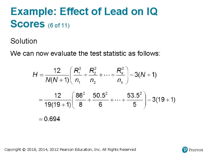
Kruskal-Wallis Test: Test Statistic Copyright © 2018, 2014, 2012 Pearson Education, Inc. All Rights Reserved

Kruskal-Wallis Test: P-Values P-values are often provided by technology. By using the test statistic H and the number of degrees of freedom (k − 1), Table A-4 can be used to find a range of values for the P-value. Copyright © 2018, 2014, 2012 Pearson Education, Inc. All Rights Reserved

Kruskal-Wallis Test: Critical Values 1. The test is right-tailed and critical values can be found from technology or from the chi-square distribution in Table A-4. 2. df = k − 1 (where df is the number of degrees of freedom and k is the number of different samples) Copyright © 2018, 2014, 2012 Pearson Education, Inc. All Rights Reserved

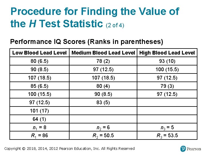
Procedure for Finding the Value of the H Test Statistic (1 of 4) Step 1: Temporarily combine all samples into one big sample and assign a rank to each sample value. (Sort the values from lowest to highest, and in cases of ties, assign to each observation the mean of the ranks involved. ) EXAMPLE: In the table on the next slide, the numbers in parentheses are the ranks of the combined data set. The rank of 1 is assigned to the lowest value of 64, the rank of 2 is assigned to the next lowest value of 78, and so on. In the case of ties, each of the tied values is assigned the mean of the ranks involved in the tie. Copyright © 2018, 2014, 2012 Pearson Education, Inc. All Rights Reserved

Procedure for Finding the Value of the H Test Statistic (2 of 4) Performance IQ Scores (Ranks in parentheses) Low Blood Lead Level Medium Blood Lead Level High Blood Lead Level 80 (6. 5) 78 (2) 93 (10) 90 (8. 5) 97 (12. 5) 100 (15. 5) 107 (18. 5) 97 (12. 5) 85 (6. 5) 80 (4) 79 (3) 100 (15. 5) 90 (8. 5) 97 (12. 5) 83 (5) Blank 101 (17) Blank 64 (1) Blank n 1 = 8 n 2 = 6 n 3 = 5 R 1 = 86 R 2 = 50. 5 R 3 = 53. 5 Copyright © 2018, 2014, 2012 Pearson Education, Inc. All Rights Reserved

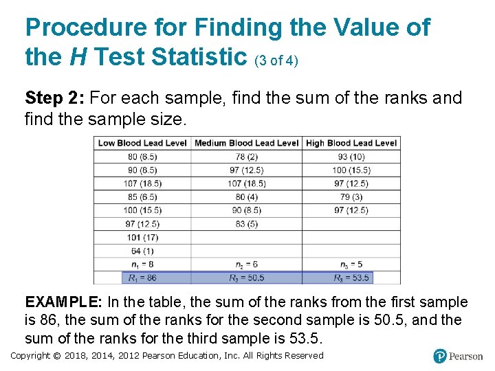
Procedure for Finding the Value of the H Test Statistic (3 of 4) Step 2: For each sample, find the sum of the ranks and find the sample size. EXAMPLE: In the table, the sum of the ranks from the first sample is 86, the sum of the ranks for the second sample is 50. 5, and the sum of the ranks for the third sample is 53. 5. Copyright © 2018, 2014, 2012 Pearson Education, Inc. All Rights Reserved

Procedure for Finding the Value of the H Test Statistic (4 of 4) Step 3: Calculate H using the results of Step 2 and the notation and test statistic given. EXAMPLE: The test statistic is computed in the next example. Copyright © 2018, 2014, 2012 Pearson Education, Inc. All Rights Reserved

Example: Effect of Lead on IQ Scores (1 of 11) The table on the next slide lists performance (nonverbal) IQ scores from samples of subjects with low blood lead level, medium blood lead level, and high blood lead level. Use a 0. 05 significance level to test the claim that the three samples of performance IQ scores come from populations with medians that are all equal. Copyright © 2018, 2014, 2012 Pearson Education, Inc. All Rights Reserved

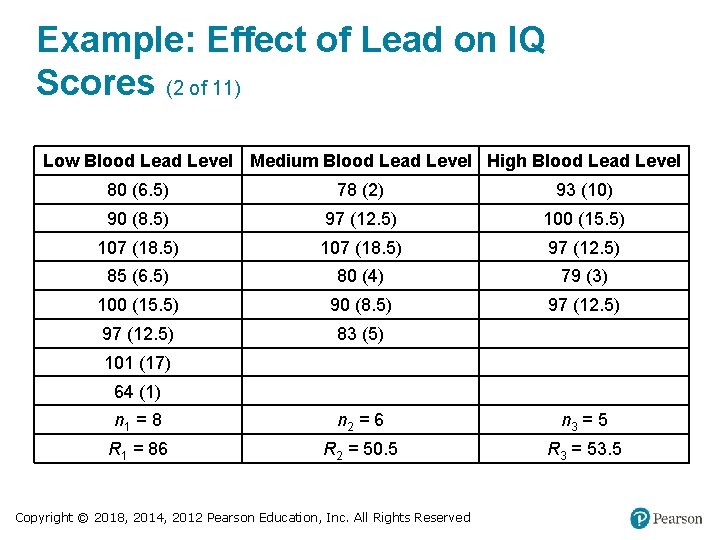
Example: Effect of Lead on IQ Scores (2 of 11) Low Blood Lead Level Medium Blood Lead Level High Blood Lead Level 80 (6. 5) 78 (2) 93 (10) 90 (8. 5) 97 (12. 5) 100 (15. 5) 107 (18. 5) 97 (12. 5) 85 (6. 5) 80 (4) 79 (3) 100 (15. 5) 90 (8. 5) 97 (12. 5) 83 (5) Blank 101 (17) Blank 64 (1) Blank n 1 = 8 n 2 = 6 n 3 = 5 R 1 = 86 R 2 = 50. 5 R 3 = 53. 5 Copyright © 2018, 2014, 2012 Pearson Education, Inc. All Rights Reserved

Example: Effect of Lead on IQ Scores (3 of 11) Solution Requirement Check (1) Each of the three samples is a simple random independent sample. (2) Each sample size is at least 5. The requirements are satisfied. Copyright © 2018, 2014, 2012 Pearson Education, Inc. All Rights Reserved

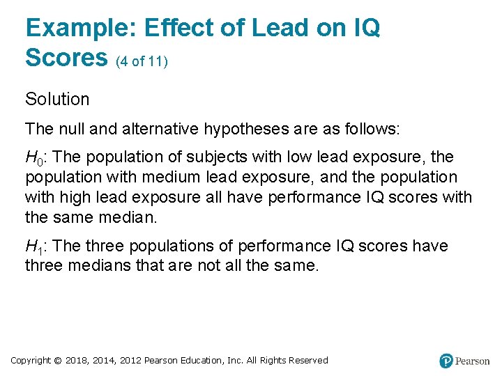
Example: Effect of Lead on IQ Scores (4 of 11) Solution The null and alternative hypotheses are as follows: H 0: The population of subjects with low lead exposure, the population with medium lead exposure, and the population with high lead exposure all have performance IQ scores with the same median. H 1: The three populations of performance IQ scores have three medians that are not all the same. Copyright © 2018, 2014, 2012 Pearson Education, Inc. All Rights Reserved

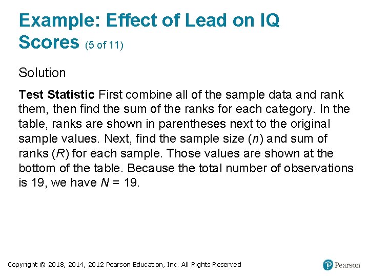
Example: Effect of Lead on IQ Scores (5 of 11) Solution Test Statistic First combine all of the sample data and rank them, then find the sum of the ranks for each category. In the table, ranks are shown in parentheses next to the original sample values. Next, find the sample size (n) and sum of ranks (R) for each sample. Those values are shown at the bottom of the table. Because the total number of observations is 19, we have N = 19. Copyright © 2018, 2014, 2012 Pearson Education, Inc. All Rights Reserved

Example: Effect of Lead on IQ Scores (6 of 11) Solution We can now evaluate the test statistic as follows: Copyright © 2018, 2014, 2012 Pearson Education, Inc. All Rights Reserved

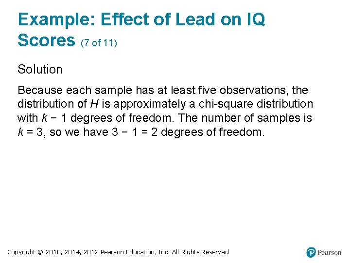
Example: Effect of Lead on IQ Scores (7 of 11) Solution Because each sample has at least five observations, the distribution of H is approximately a chi-square distribution with k − 1 degrees of freedom. The number of samples is k = 3, so we have 3 − 1 = 2 degrees of freedom. Copyright © 2018, 2014, 2012 Pearson Education, Inc. All Rights Reserved

Example: Effect of Lead on IQ Scores (8 of 11) Solution P-Value With H = 0. 694 and df = 2, Table A-4 shows that the P-value is greater than 0. 10. Using technology, we get P-value = 0. 707. Because the P-value is greater than the significance level of 0. 05, we fail to reject the null hypothesis of equal population medians. Copyright © 2018, 2014, 2012 Pearson Education, Inc. All Rights Reserved

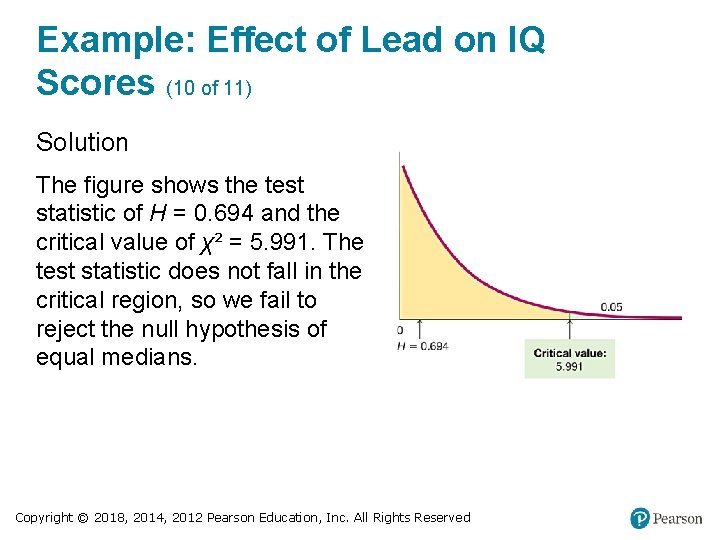
Example: Effect of Lead on IQ Scores (9 of 11) Solution Critical Value Refer to Table A-4 to find the critical value of 5. 991, which corresponds to 2 degrees of freedom and a 0. 05 significance level (with an area of 0. 05 in the right tail). The figure on the next slide shows that the test statistic H = 0. 694 does not fall within the critical region bounded by 5. 991, so we fail to reject the null hypothesis of equal population medians. Copyright © 2018, 2014, 2012 Pearson Education, Inc. All Rights Reserved

Example: Effect of Lead on IQ Scores (10 of 11) Solution The figure shows the test statistic of H = 0. 694 and the critical value of χ² = 5. 991. The test statistic does not fall in the critical region, so we fail to reject the null hypothesis of equal medians. Copyright © 2018, 2014, 2012 Pearson Education, Inc. All Rights Reserved

Example: Effect of Lead on IQ Scores (11 of 11) Interpretation There is not sufficient evidence to reject the claim that the three samples of performance IQ scores come from populations with medians that are all equal. The population medians do not appear to be significantly different. Copyright © 2018, 2014, 2012 Pearson Education, Inc. All Rights Reserved