Computational Learning Theory 1 A theory of the

Computational Learning Theory 1

A theory of the learnable (Valiant ‘ 84) p […] The problem is to discover good models that are interesting to study for their own sake and that promise to be relevant both to explaining human experience and to building devices that can learn […] Learning machines must have all 3 of the following properties: l the machines can provably learn whole classes of concepts, these classes can be characterized l the classes of concepts are appropriate and nontrivial for generalpurpose knowledge l the computational process by which the machine builds the desired programs requires a “feasible” (i. e. polynomial) number of steps 2

A theory of the learnable p We seek general laws that constrain inductive learning, relating: l Probability of successful learning l Number of training examples l Complexity of hypothesis space l Accuracy to which target concept is approximated l Manner in which training examples are presented 3

Overview p Are there general laws that govern learning? l l l p Sample Complexity: How many training examples are needed for a learner to converge (with high probability) to a successful hypothesis? Computational Complexity: How much computational effort is needed for a learner to converge (with high probability) to a successful hypothesis? Mistake Bound: How many training examples will the learner misclassify before converging to a successful hypothesis? These questions will be answered within two analytical frameworks: l l The Probably Approximately Correct (PAC) framework The Mistake Bound framework 4

Overview (Cont’d) p Rather than answering these questions for individual learners, we will answer them for broad classes of learners. In particular we will consider: l l The size or complexity of the hypothesis space considered by the learner. The accuracy to which the target concept must be approximated. The probability that the learner will output a successful hypothesis. The manner in which training examples are presented to the learner. 5

Introduction p Problem setting l p Inductively learning an unknown target function, given training examples and a hypothesis space Focus on: l l How many training examples are sufficient? How many mistakes will the learner make before it succeeds? 6

Introduction (2) p Desirable: quantitative bounds depending on l l Complexity of hypo space, Accuracy of approximation to the target Probability of outputting a successful hypo How the training examples are presented n n n p Learner proposes instances Teacher presents instances Some random process produces instances Specifically, study sample complexity, computational complexity, and mistake bound. 7

Problem Setting p p ü Space of possible instances X (e. g. set of all people) over which target functions may be defined. Assume that different instances in X may be encountered with different frequencies. Modeling above assumption as: unknown (stationary) probability distribution D that defines the probability of encountering each instance in X Training examples are provided by drawing instances independently from X, according to D, and they are noise-free. Each element c in target function set C corresponds to certain subset of X, i. e. c is a Boolean function. (Just for the sake of simplicity) 8

Error of a Hypothesis p p p Training error of hypo h w. r. t. target function c and training data set S of n sample is True error of hypo h w. r. t. target function c and distribution D is error. D(h) is not observable, so how probable is it that error. S(h) gives a misleading estimates of error. D(h)? l Different from problem setting in Ch 5, where samples are drawn independently from h, here h depends on training samples. 9

An Illustration of True Error 10

Theoretical Questions of Interest p p p Is it possible to identify classes of learning problems that are inherently difficult or easy, independent of the learning algorithm? Can one characterize the number of training examples necessary or sufficient to assure successful learning? How is the number of examples affected l l p p If observing a random sample of training data? if the learner is allowed to pose queries to the trainer? Can one characterize the number of mistakes that a learner will make before learning the target function? Can one characterize the inherent computational complexity of a class of learning algorithms?

Computational Learning Theory p p Relatively recent field Area of intense research Partial answers to some questions on previous page is yes. Will generally focus on certain types of learning problems.

Inductive Learning of Target Function p What we are given l l p Hypothesis space Training examples What we want to know l l How many training examples are sufficient to successfully learn the target function? How many mistakes will the learner make before succeeding?

Computational Learning Theory Provides a theoretical analysis of learning: p p Is it possible to identify classes of learning problems that are inherently difficult/easy? Can we characterize the computational complexity of classes of learning problems • • p Can we characterize the number of training samples necessary/sufficient for successful learning? l p When a learning algorithm can be expected to succeed When learning may be impossible How is this number affected if we allow the learner to ask questions (active learning) How many mistakes will the learner make before learning the target function

p Computational Learning Theory Quantitative bounds can be set depending on the following attributes: p p Accuracy to which the target must be approximated The probability that the learner will output a successful hypothesis Size or complexity of the hypothesis space considered by the learner The manner in which training examples are presented to the learner

Computational Learning Theory Three general areas: 1. 2. 3. Sample Complexity. How many examples we need to find a good hypothesis? Computational Complexity. How much computational power we need to find a good hypothesis? Mistake Bound. How many mistakes we will make before finding a good hypothesis?

p Sample Complexity How Many Training Examples Sufficient To Learn Target Concept? Scenario 1: Active Learning Learner proposes instances, as queries to teacher Query (learner): instance x Answer (teacher): c(x) Scenario 2: Passive Learning from Teacher-Selected Examples Teacher (who knows c) provides training examples Sequence of examples (teacher): {<xi, c(xi)>} Teacher may or may not be helpful, optimal Scenario 3: Passive Learning from Teacher-Annotated Examples Random process (e. g. , nature) proposes instances Instance x generated randomly, teacher provides c(x)

Models of Learning p p p Learner: who is doing the learning? (e. g. A computer with limited resources (finite memory, polynomial time, . . . ) Domain: What is being learnt? (e. g. Concept of a chair) Information source: - Examples - positive/negative - according to a certain distribution - selected how? - features? Queries - “is this a chair? ” - Experimentation - play with a new gadget to learn how it works l Noisy or noise-free? p p Prior knowledge: e. g. “The concept to learn is a conjunction of features” Performance criteria: - Measure of how well learned? Done? Accuracy (error rate) Efficiency

Computational Learning Theory • The PAC Learning Framework • Finite Hypothesis Spaces • • p Examples of PAC Learnable Concepts VC dimension & Infinite Hyp. Spaces The Mistake Bound Model

Two Frameworks p PAC (Probably Approximately Correct) Learning Framework: Identify classes of hypotheses that can and cannot be learned from a polynomial number of training examples l p Define a natural measure of complexity for hypothesis spaces that allows bounding the number of training examples needed Mistake Bound Framework

PAC Learning p p Probably Approximately Correct Learning Model Will restrict discussion to learning booleanvalued concepts in noise-free data.

Problem Setting: Instances and Concepts p p X is set of all possible instances over which target function may be defined C is set of target concepts learner is to learn l l Each target concept c in C is a subset of X Each target concept c in C is a boolean function c: X {0, 1} c(x) = 1 if x is positive example of concept c(x) = 0 otherwise

Problem Setting: Distribution p Instances generated at random using some probability distribution D l l l p D may be any distribution D is generally not known to the learner D is required to be stationary (does not change over time) Training examples x are drawn at random from X according to D and presented with target value c(x) to the learner.

Problem Setting: Hypotheses p p Learner L considers set of hypotheses H After observing a sequence of training examples of the target concept c, L must output some hypothesis h from H which is its estimate of c

Example Problem (Classifying Executables) p p Three Classes (Malicious, Boring, Funny) Features l l p p a 1 a 2 a 3 a 4 GUI present (yes/no) Deletes files (yes/no) Allocates memory (yes/no) Creates new thread (yes/no) Distribution? Hypotheses?

Instance a 1 a 2 a 3 a 4 Class 1 Yes No No Yes B 2 Yes No No No B 3 No Yes No F 4 No No Yes M 5 Yes No No Yes B 6 Yes No No No F 7 Yes Yes No M 8 Yes No Yes M 9 No No No Yes B 10 No No Yes No M

True Error p Definition: The true error (denoted error. D(h)) of hypothesis h with respect to target concept c and distribution D , is the probability that h will misclassify an instance drawn at random according to D. Computer Science Department CS 9633 Machine Learning

Error of h with respect to c p p - p Instance space X p p c p + p p + + p p h - Computer Science Department CS 9633 Machine Learning -

Key Points p p True error defined over entire instance space, not just training data Error depends strongly on the unknown probability distribution D The error of h with respect to c is not directly observable to the learner L—can only observe performance with respect to training data (training error) Question: How probable is it that the observed training error for h gives a misleading estimate of the true error? Computer Science Department CS 9633 Machine Learning

PAC Learnability p Goal: characterize classes of target concepts that can be reliably learned l l p from a reasonable number of randomly drawn training examples and using a reasonable amount of computation Unreasonable to expect perfect learning where error. D(h) = 0 l l Would need to provide training examples corresponding to every possible instance With random sample of training examples, there is always a non-zero probability that the training examples will be misleading Computer Science Department CS 9633 Machine Learning

Weaken Demand on Learner p Hypothesis error (Approximately) l l l p Will not require a zero error hypothesis Require that error is bounded by some constant , that can be made arbitrarily small is the error parameter Error on training data (Probably) l l l Will not require that the learner succeed on every sequence of randomly drawn training examples Require that its probability of failure is bounded by a constant, , that can be made arbitrarily small is the confidence parameter Computer Science Department CS 9633 Machine Learning

Probably Approximately Correct Learning (PAC Learning) 34

Computational Learning Theory Three general areas: 1. 2. 3. Sample Complexity. How many examples we need to find a good hypothesis? Computational Complexity. How much computational power we need to find a good hypothesis? Mistake Bound. How many mistakes we will make before finding a good hypothesis?

Two Frameworks p PAC (Probably Approximately Correct) Learning Framework: Identify classes of hypotheses that can and cannot be learned from a polynomial number of training examples l p Define a natural measure of complexity for hypothesis spaces that allows bounding the number of training examples needed Mistake Bound Framework

Cannot Learn Exact Concepts from Limited Data, Only Approximations p p Positive Negative p Learner p Classifier Positive Negative p p 37

Cannot Learn Even Approximate Concepts from Pathological Training Sets p p Positive Negative p Learner p Classifier Positive Negative p 38

Probably approximately correct learning formal computational model which want shed light on the limits of what can be learned by a machine, analysing the computational cost of learning algorithms 39

What we want to learn CONCEPT = recognizing algorithm p LEARNING = computational description of recognizing algorithms starting from: - examples - incomplete specifications That is: to determine uniformly good approximations of an unknown function from its value in some sample points p interpolation p pattern matching p concept learning 40

What’s new in p. a. c. learning? Accuracy of results and running time for learning algorithms are explicitly quantified and related A general problem: use of resources (time, space…) by computations Example Sorting: Bool. satisfiability: COMPLEXITY THEORY n·logn time (polynomial, feasible) 2ⁿ time (exponential, intractable) 41

PAC Learnability p p PAC refers to Probably Approximately Correct It is desirable that error. D(h) to be zero, however, to be realistic, we weaken our demand in two ways: l l p error. D(h) is to be bounded by a small number ε Learner is not required to success on every training sample, rather that its probability of failure is to be bounded by a constant δ. Hence we come up with the idea of “Probably Approximately Correct” 42

PAC Learning p p The only reasonable expectation of a learner is that with high probability it learns a close approximation to the target concept. In the PAC model, we specify two small parameters, ε and δ, and require that with probability at least (1 δ) a system learn a concept with error at most ε. 43

The PAC Learning Framework Definition: A class of concepts C is PAC learnable using a hypothesis class H, if there exist a learning algorithm L such that for arbitrary small δ and ε, and for all concepts c in C, and for all distributions D over the input space, there is a 1 -δ probability that the hypothesis h selected from space H by L is approximately correct (has less than ε true error). p

Definition of PACLearnability p p Definition: Consider a concept class C defined over a set of instances X of length n and a learner L using hypothesis space H. C is PAC-learnable by L using H if all c C, distributions D over X, such that 0 < < ½ , and such that 0 < < ½, learner L will with probability at least (1 - ) output a hypothesis h H such that error. D(h) , in time that is polynomial in 1/ , n, and size(c). Computer Science Department CS 9633 Machine Learning

Requirements of Definition p p L must with arbitrarily high probability (1 - ), out put a hypothesis having arbitrarily low error ( ). L’s learning must be efficient—grows polynomially in terms of l l Strengths of output hypothesis (1/ , 1/ ) Inherent complexity of instance space (n) and concept class C (size(c)). Computer Science Department CS 9633 Machine Learning

Block Diagram of PAC Learning Model Control Parameters p , p Training sample p p Learning algorithm L p Computer Science Department CS 9633 Machine Learning Hypothesis p h

Examples of second requirement p Consider executables problem where instances are conjunctions of boolean features: a 1=yes a 2=no a 3=yes a 4=no p Concepts are conjunctions of a subset of the features a 1=yes a 3=yes a 4=yes

Using the Concept of PAC Learning in Practice p p We often want to know how many training instances we need in order to achieve a certain level of accuracy with a specified probability. If L requires some minimum processing time per training example, then for C to be PAClearnable by L, L must learn from a polynomial number of training examples. Computer Science Department CS 9633 Machine Learning

Sample Complexity for Finite Hypothesis Spaces 50

Sample Complexity for Finite Hypothesis Spaces p p p Start from a good class of learner—consistent learner, defined as one that outputs a hypo which perfectly fits the training data set, whenever possible. Recall: Version space VSH, D is defined to be the set of all hypo h∈H that correctly classify all training examples in D. Property. Every consistent learner outputs a hypo belonging to version space. 51

Sample Complexity for Finite Hypothesis Spaces p p Given any consistent learner, the number of examples sufficient to assure that any hypothesis will be probably (with probability (1 - )) approximately (within error ) correct is m= 1/ (ln|H|+ln(1/ )) If the learner is not consistent, m= 1/2 2 (ln|H|+ln(1/ )) Conjunctions of Boolean Literals are also PACLearnable and m= 1/ (n. ln 3+ln(1/ )) k-term DNF expressions are not PAC learnable because even though they have polynomial sample complexity, their computational complexity is not 52

Formal Definition of PACLearnable p p Consider a concept class C defined over an instance space X containing instances of length n, and a learner, L, using a hypothesis space, H. C is said to be PAC-learnable by L using H iff for all c C, distributions D over X, 0<ε<0. 5, 0<δ<0. 5; learner L by sampling random examples from distribution D, will with probability at least 1 δ output a hypothesis h H such that error. D(h) ε, in time polynomial in 1/ε, 1/δ, n and size(c). Example: l l l X: instances described by n binary features C: conjunctive descriptions over these features H: conjunctive descriptions over these features L: most-specific conjunctive generalization algorithm (Find-S) size(c): the number of literals 53 in c (i. e. length of the conjunction).

ε-exhausted p Def. VSH, D is said to be ε-exhausted w. r. t. c and D if for any h in VSH, D, error. D(h)<ε. 54

A PAC-Learnable Example p Consider class C of conjunction of boolean literals. l p p A boolean literal is any boolean variable or its negation Q: Is such C PAC-learnable? A: Yes, by going through the following two steps: 1. 2. Show that any consistent learner will require only a polynomial number of training examples to learn any element of C Suggest a specific algorithm that use polynomial time per training example. 55

Contd Step 1: p Let H consist of conjunction of literals based on n boolean variables. p Now take a look at m≥(1/ε)(ln|H|+ln(1/δ)), observe that |H|=3 n, then the inequality becomes m≥(1/ε)(nln 3+ln(1/δ)). Step 2: p FIND-S algorithm satisfies the requirement l For each new positive training example, the algorithm computes intersection of literals shared by current hypothesis and the example, using time linear in n 56

p Sample Complexity of Conjunction Learning Consider conjunctions over n boolean features. There are 3 n of these since each feature can appear positively, appear negatively, or not appear in a given conjunction. Therefore |H|= 3 n, so a sufficient number of examples to learn a PAC concept is: p p Concrete examples: l δ=ε=0. 05, n=10 gives 280 examples l δ=0. 01, ε=0. 05, n=10 gives 312 examples l δ=ε=0. 01, n=10 gives 1, 560 examples l δ=ε=0. 01, n=50 gives 5, 954 examples Result holds for any consistent learner, including Find. S. 57

p Sample Complexity of Learning Arbitrary Boolean Consider any boolean function. Functions over n boolean features such as the hypothesis space of DNF or decision trees. There are 2 2^n of these, so a sufficient number of examples to learn a PAC concept is: p Concrete examples: l δ=ε=0. 05, n=10 gives 14, 256 examples l δ=ε=0. 05, n=20 gives 14, 536, 410 examples 16 examples l δ=ε=0. 05, n=50 gives 1. 561 x 10 58

Agnostic Learning & Inconsistent Hypo p p we assume that VSH, D is not empty, and a simple way to guarantee such condition holds is that we assume that c belongs to H. Agnostic learning setting: Don’t assume c∈H, and the learner simply finds hypo with minimum training error instead. 59

Sample Complexity for Infinite Hypothesis Spaces 60

Infinite Hypothesis Spaces p p The preceding analysis was restricted to finite hypothesis spaces. Some infinite hypothesis spaces (such as those including real-valued thresholds or parameters) are more expressive than others. l p p p Compare a rule allowing one threshold on a continuous feature (length<3 cm) vs one allowing two thresholds (1 cm<length<3 cm). Need some measure of the expressiveness of infinite hypothesis spaces. The Vapnik-Chervonenkis (VC) dimension provides just such a measure, denoted VC(H). Analagous to ln|H|, there are bounds for sample complexity using VC(H). 61

p p p VC Dimension An unbiased hypothesis space shatters the entire instance space. The larger the subset of X that can be shattered, the more expressive the hypothesis space is, i. e. the less biased. The Vapnik-Chervonenkis dimension, VC(H). of hypothesis space H defined over instance space X is the size of the largest finite subset of X shattered by H. If arbitrarily large finite subsets of X can be shattered then VC(H) = If there exists at least one subset of X of size d that can be shattered then VC(H) ≥ d. If no subset of size d can be shattered, then VC(H) < d. For a single intervals on the real line, all sets of 2 instances can be shattered, but no set of 3 instances can, so VC(H) = 2. 62

Shattering a Set of Instances p p Def. A dichotomy of a set S is a partition of S into two disjoint subsets Def. A set of instances S is shattered by hypo space H iff for every dichotomy of S, there exists some hypo in H consistent with this dichotomy. 3 instances shattered 63

p VC Dimension We say that a set S of examples is shattered by a set of functions H if p for every partition of the examples in S into positive and negative examples p there is a function in H that gives exactly these labels to the examples • The VC dimension of hypothesis space H over instance space X p is the size of the largest finite subset of X that is shattered by H. • p • • If there exists a subset of size d can be shattered, then VC(H) >=d If no subset of size d can be shattered, then VC(H) < d VC(Half intervals) = 1 p. VC( Intervals) = 2 p. VC(Half-spaces in the plane) = 3 p Computational Learning Theory (no subset of size 2 can be shattered) (no subset of size 3 can be shattered) (no subset of size 4 can be shattered) CS 446 -Spring 06 64

VC Dimension p p Motivation: What if H can’t shatter X? Try finite subsets of X. Def. VC dimension of hypo space H defined over instance space X is the size of largest finite subset of X shattered by H. If any arbitrarily large finite subsets of X can be shattered by H, then VC(H)≡∞ Roughly speaking, VC dimension measures how many (training) points can be separated for all possible labeling using functions of a given class. Notice that for any finite H, VC(H)≤log 2|H| 65

Sample Complexity for Infinite Hypothesis Spaces II p p Upper-Bound on sample complexity, using the VCDimension: m 1/ (4 log 2(2/ )+8 VC(H)log 2(13/ ) Lower Bound on sample complexity, using the VCDimension: Consider any concept class C such that VC(C) 2, any learner L, and any 0 < < 1/8, and 0 < < 1/100. Then there exists a distribution D and target concept in C such that if L observes fewer examples than max[1/ log(1/ ), (VC(C)-1)/(32 )] then with probability at least , L outputs a hypothesis h having error. D(h)> . 66

An Example: Linear Decision Surface p p p Line case: X=real number set, and H=set of all open intervals, then VC(H)=2. Plane case: X=xy-plane, and H=set of all linear decision surface of the plane, then VC(H)=3. General case: For n-dim real-number space, let H be its linear decision surface, then VC(H)=n+1. 67

Sample Complexity from VC Dimension How many randomly drawn examples suffice to ε-exhaust VSH, D with probability at least 1 -δ? (Blumer et al. 1989) p Furthermore, it is possible to obtain a lower bound on sample complexity (i. e. minimum number of required training samples) p 68

Lower Bound on Sample Complexity p Theorem 7. 2 (Ehrenfeucht et al. 1989) Consider any concept class C s. t. VC(C)≥ 2, any learner L, and any 0<ε<1/8, and 0<δ<1/100. Then there exists a distribution D and target concept in C s. t. if L observes fewer examples than max[(1/ε)log(1/δ), (VC(C)-1)/(32ε)], then with probability at least δ, L outputs a hypo h having error. D(h)>ε. 69

VC-Dimension for Neural Networks p p Let G be a layered directed acyclic graph with n input nodes and s 2 internal nodes, each having at most r inputs. Let C be a concept class over Rr of VC dimension d, corresponding to the set of functions that can be described by each of the s internal nodes. Let CG be the G-composition of C, corresponding to the set of functions that can be represented by G. Then VC(CG) 2 ds log(es), where e is the base of the natural logarithm. This theorem can help us bound the VC-Dimension of a neural network and thus, its sample complexity 70

Mistake Bound Model 71

Mistake Bound Model p The learner receives a sequence of training examples • p Upon receiving each example x, the learner must predict the target value c(x) • p Instance based learning Online learning How many mistakes will the learner make before it learns the target concept? • e. g. Learning fraudulent credit card purchases

Mistake Bound Model

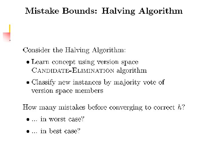
p p p When the majority of the hypotheses incorrectly classifies the new example, the VS will be reduced to at most half its current size Given that the VS initially contains |H| hypotheses, the maximum number of mistakes possible before VS contains just one member is log 2|H| The algorithm can learn without any mistakes at all l when the majority is correct, it will remove the incorrect, minority hypotheses

Skip p We may also ask what is the Optimal Mistake bound (Opt(C))? l l lowest worst-case mistake bound over all possible learning algorithms VC(C) < Opt(C) < MHalving(C) < log 2|C|

Introduction (2) p Desirable: quantitative bounds depending on l l Complexity of hypo space, Accuracy of approximation Probability of outputting a successful hypo How the training examples are presented n n n p Learner proposes instances Teacher presents instances Some random process produces instances Specifically, study sample complexity, computational complexity, and mistake bound. 76

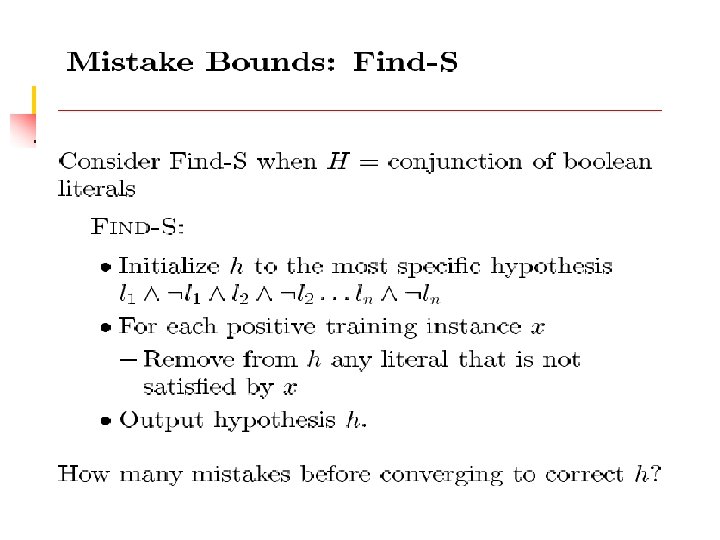
Introduction to “Mistake Bound” p p p Mistake bound: the total number of mistakes a learner makes before it converges to the correct hypothesis Assume the learner receives a sequence of training examples, however, for each instance x, the learner must first predict c(x) before it receives correct answer from the teacher. Application scenario: when the learning must be done on-the-fly, rather than during off-line training stage. 77

The Mistake Bound Model of Learning p p The Mistake Bound framework is different from the PAC framework as it considers learners that receive a sequence of training examples and that predict, upon receiving each example, what its target value is. The question asked in this setting is: “How many mistakes will the learner make in its predictions before it learns the target concept? ” p This question is significant in practical settings where learning must be done while the system is in actual use. 78

Theorem 1. Online learning of conjunctive concepts can be done with p at most n+1 prediction mistakes.

Find-S Algorithm Finding-S: Find a maximally specific hypothesis 1. Initialize h to the most specific hypothesis in H 2. For each positive training example x l 3. For each attribute constraint ai in h, if it is satisfied by x, then do nothing; otherwise replace ai by the next more general constraint that is satisfied by x. Output hypo h 81

Mistake Bound for FIND-S p p Assume training data is noise-free and target concept c is in the hypo space H, which consists of conjunction of up to n boolean literals Then in the worst case the learner needs to make n+1 mistakes before it learns c l l Note that misclassification occurs only in case that the latest learned hypo misclassifies a positive example as negative, and one such mistake removes at least one constraint from the hypo, and in the above worst case, c is the function that assigns every instance to “true” value 82

Mistake Bound for Halving Algorithm p p Halving algorithm = incrementally learning the version space as every new instance arrives + predict a new instance by majority votes (of hypo in VS) Q: What is the maximum number of mistakes that can be made by a halving algorithm, for an arbitrary finite H, before it exactly learns the target concept c (assume c is in H)? l p Answer: the largest integer no more than log 2|H| How about the minimum number of mistakes? l Answer: zero-mistake! 84

Optimal Mistake Bounds p p For an arbitrary concept class C, assuming H=C, interested in the lowest worst-case mistake bound over all possible learning algorithms Let MA(c) denotes the maximum number of mistakes over all possible training examples that a learner A makes to exactly learn c. Def. MA(C) ≡maxc∈CMA(c) Ex: MFIND-s(C)=n+1, MHalving(C)≤log 2|C| 85

Optimal Mistake Bounds (2) p p The optimal mistake bound for C, denoted by Opt(C), defined as min. A∈learning alg. MA(C) Notice that Opt(C)≤MHalving(C)≤log 2|C| Furthermore, Littlestone (1987) shows that VC(C)≤Opt(C) ! When C equal to the power-set Cp of any finite instance space X, the above four quantities become equal to each other, i. e. |X | 86

Optimal Mistake Bounds p p Definition: Let C be an arbitrary nonempty concept class. The optimal mistake bound for C, denoted Opt(C), is the minimum over all possible learning algorithms A of MA(C). Opt(C)=min. A Learning_Algorithm MA(C) For any concept class C, the optimal mistake bound is bound as follows: VC(C) Opt(C) log 2(|C|) 87

Weighted-Majority Algorithm p p It is a generalization of Halving algorithm: makes a prediction by taking a weighted vote among a pool of prediction algorithms (or hypotheses) and learns by altering the weights It starts by assigning equal weight (=1) to every prediction algorithm. Whenever an algorithm misclassifies a training example, reduces its weight l Halving algorithm reduces the weight to zero 88

Procedure for Adjusting Weights ai denotes the ith prediction algorithm in the pool; wi denotes the weight of ai, and is initialized to 1 p For each training example <x, c(x)> l l l Initialize q 0 & q 1 to be 0 For each ai, if ai(x)=0 then q 0←q 0+wi, else q 1←q 1+wi If q 1>q 0, predicts c(x) to be 1, else n n l if q 1<q 0, predicts c(x) to be 0, else predicts c(x) at random to be 1 or 0. For each ai, do n If ai(x)≠c(x) (given by the teacher), wi←βwi 89

A Case Study: The Weighted. Majority Algorithm ai denotes the ith prediction algorithm in the pool A of algorithm. wi denotes the weight associated with ai. p For all i initialize wi <-- 1 p For each training example <x, c(x)> l l Initialize q 0 and q 1 to 0 For each prediction algorithm ai If ai(x)=0 then q 0 <-- q 0+wi n If ai(x)=1 then q 1 <-- q 1+wi n l l If q 1 > q 0 then predict c(x)=1 If q 0 > q 1 then predict c(x) =0 If q 0=q 1 then predict 0 or 1 at random for c(x) For each prediction algorithm ai in A do n If ai(x) c(x) then wi <-- wi 90

Comments on “Adjusting Weights” Idea p p The idea can be found in various problems such as pattern matching, where we might reduce weights of less frequently used patterns in the learned library The textbook claims that one benefit of the algorithm is that it is able to accommodate inconsistent training data, but in case of learning by query, we presume that answer given by the teacher is always correct. 91

Relative Mistake Bound for the Algorithm p p Theorem 7. 3 Let D be the training sequence, A be any set of n prediction algorithms, and k be the minimum number of mistakes made by any algorithm in A for the training sequence D. Then the number of mistakes over D made by Weighted-Majority algorithm using β=0. 5 is at most 2. 4(k+log 2 n) Proof: The basic idea is that we compare the final weight of best prediction algorithm to the sum of weights over all predictions. Let aj be such algorithm with k mistakes, then its final weight wj=0. 5 k. Now consider the sum W of weights over all predictions, observe that for every mistake made, W is reduced to at most 0. 75 W. 92

Relative Mistake Bound for the Weighted-Majority Algorithm p Let D be any sequence of training examples, let A be any set of n prediction algorithms, and let k be the minimum number of mistakes made by any algorithm in A for the training sequence D. Then the number of mistakes over D made by the Weighted. Majority algorithm using =1/2 is at most 2. 4(k + log 2 n). p This theorem can be generalized for any 0 1 where the bound becomes (k log 2 1/ + log 2 n)/log 2(2/(1+ )) 93