Natural Language Processing Chapter 19 Computational Lexical Semantics

Natural Language Processing Chapter 19 Computational Lexical Semantics Part 2 [Includes slides from a AAAI-2005 tutorial by Rada Mihalcea and Ted Pedersen]

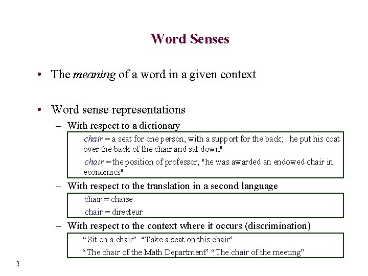
Word Senses • The meaning of a word in a given context • Word sense representations – With respect to a dictionary chair = a seat for one person, with a support for the back; "he put his coat over the back of the chair and sat down" chair = the position of professor; "he was awarded an endowed chair in economics" – With respect to the translation in a second language chair = chaise chair = directeur – With respect to the context where it occurs (discrimination) “Sit on a chair” “Take a seat on this chair” “The chair of the Math Department” “The chair of the meeting” 2

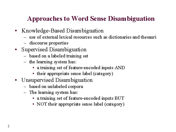
Approaches to Word Sense Disambiguation • Knowledge-Based Disambiguation – use of external lexical resources such as dictionaries and thesauri – discourse properties • Supervised Disambiguation – based on a labeled training set – the learning system has: • a training set of feature-encoded inputs AND • their appropriate sense label (category) • Unsupervised Disambiguation – based on unlabeled corpora – The learning system has: • a training set of feature-encoded inputs BUT • NOT their appropriate sense label (category) 3

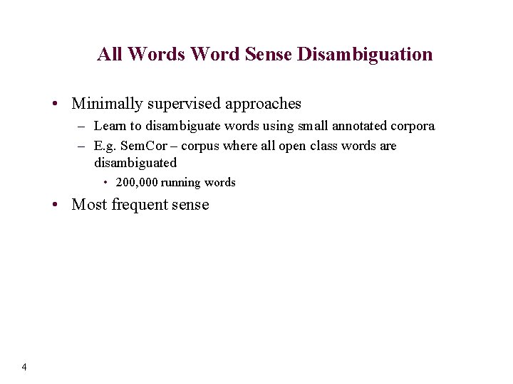
All Words Word Sense Disambiguation • Minimally supervised approaches – Learn to disambiguate words using small annotated corpora – E. g. Sem. Cor – corpus where all open class words are disambiguated • 200, 000 running words • Most frequent sense 4

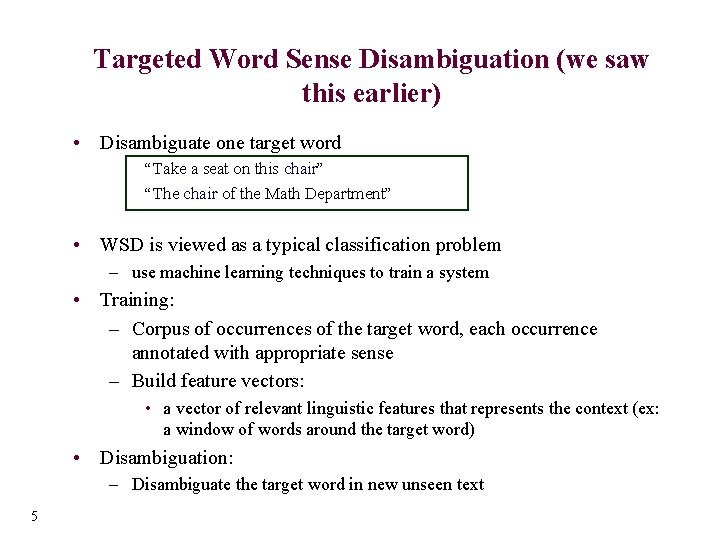
Targeted Word Sense Disambiguation (we saw this earlier) • Disambiguate one target word “Take a seat on this chair” “The chair of the Math Department” • WSD is viewed as a typical classification problem – use machine learning techniques to train a system • Training: – Corpus of occurrences of the target word, each occurrence annotated with appropriate sense – Build feature vectors: • a vector of relevant linguistic features that represents the context (ex: a window of words around the target word) • Disambiguation: – Disambiguate the target word in new unseen text 5

Knowledge-based Methods for Word Sense Disambiguation

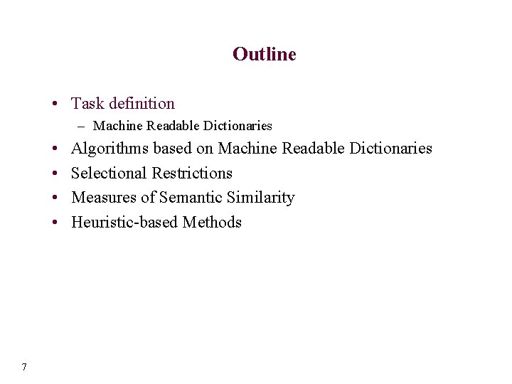
Outline • Task definition – Machine Readable Dictionaries • • 7 Algorithms based on Machine Readable Dictionaries Selectional Restrictions Measures of Semantic Similarity Heuristic-based Methods

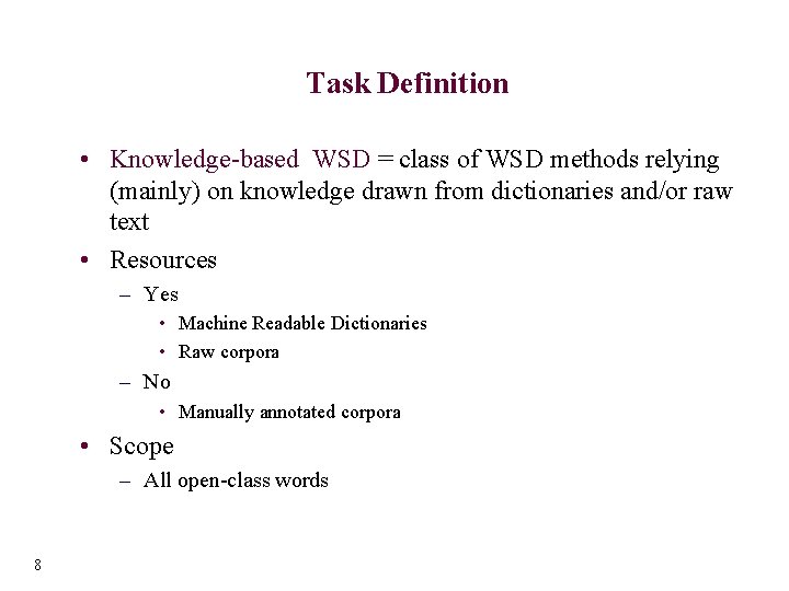
Task Definition • Knowledge-based WSD = class of WSD methods relying (mainly) on knowledge drawn from dictionaries and/or raw text • Resources – Yes • Machine Readable Dictionaries • Raw corpora – No • Manually annotated corpora • Scope – All open-class words 8

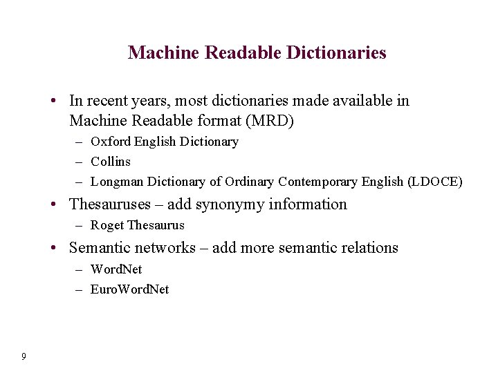
Machine Readable Dictionaries • In recent years, most dictionaries made available in Machine Readable format (MRD) – Oxford English Dictionary – Collins – Longman Dictionary of Ordinary Contemporary English (LDOCE) • Thesauruses – add synonymy information – Roget Thesaurus • Semantic networks – add more semantic relations – Word. Net – Euro. Word. Net 9

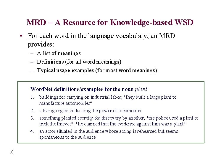
MRD – A Resource for Knowledge-based WSD • For each word in the language vocabulary, an MRD provides: – A list of meanings – Definitions (for all word meanings) – Typical usage examples (for most word meanings) Word. Net definitions/examples for the noun plant 1. buildings for carrying on industrial labor; "they built a large plant to manufacture automobiles“ 2. a living organism lacking the power of locomotion 3. something planted secretly for discovery by another; "the police used a plant to trick the thieves"; "he claimed that the evidence against him was a plant" 4. an actor situated in the audience whose acting is rehearsed but seems spontaneous to the audience 10

MRD – A Resource for Knowledge-based WSD • A thesaurus adds: – An explicit synonymy relation between word meanings Word. Net synsets for the noun “plant” 1. plant, works, industrial plant 2. plant, flora, plant life • A semantic network adds: – Hypernymy/hyponymy (IS-A), meronymy/holonymy (PART-OF), antonymy, entailnment, etc. 11 Word. Net related concepts for the meaning “plant life” {plant, flora, plant life} hypernym: {organism, being} hypomym: {house plant}, {fungus}, … meronym: {plant tissue}, {plant part} holonym: {Plantae, kingdom Plantae, plant kingdom}

Outline • Task definition – Machine Readable Dictionaries • • 12 Algorithms based on Machine Readable Dictionaries Selectional Restrictions Measures of Semantic Similarity Heuristic-based Methods

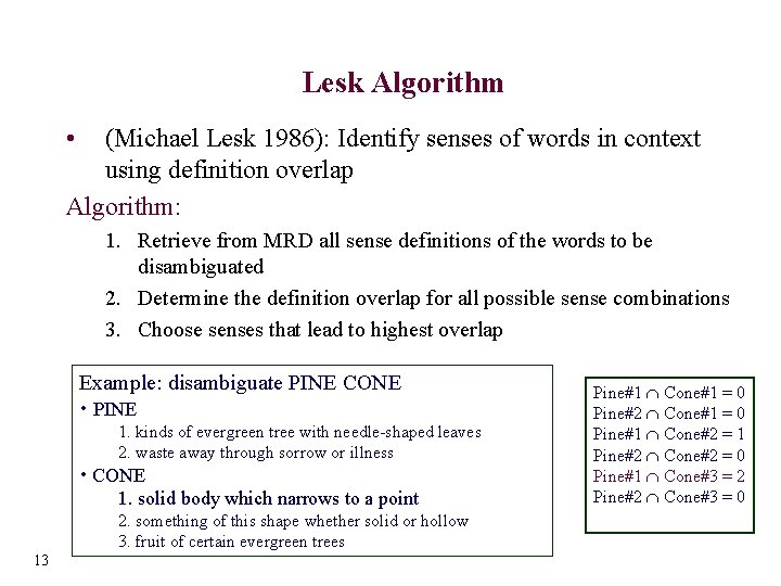
Lesk Algorithm • (Michael Lesk 1986): Identify senses of words in context using definition overlap Algorithm: 1. Retrieve from MRD all sense definitions of the words to be disambiguated 2. Determine the definition overlap for all possible sense combinations 3. Choose senses that lead to highest overlap Example: disambiguate PINE CONE • PINE 1. kinds of evergreen tree with needle-shaped leaves 2. waste away through sorrow or illness • CONE 1. solid body which narrows to a point 2. something of this shape whether solid or hollow 3. fruit of certain evergreen trees 13 Pine#1 Cone#1 = 0 Pine#2 Cone#1 = 0 Pine#1 Cone#2 = 1 Pine#2 Cone#2 = 0 Pine#1 Cone#3 = 2 Pine#2 Cone#3 = 0

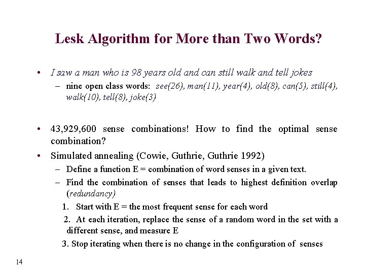
Lesk Algorithm for More than Two Words? • I saw a man who is 98 years old and can still walk and tell jokes – nine open class words: see(26), man(11), year(4), old(8), can(5), still(4), walk(10), tell(8), joke(3) • 43, 929, 600 sense combinations! How to find the optimal sense combination? • Simulated annealing (Cowie, Guthrie 1992) – Define a function E = combination of word senses in a given text. – Find the combination of senses that leads to highest definition overlap (redundancy) 1. Start with E = the most frequent sense for each word 2. At each iteration, replace the sense of a random word in the set with a different sense, and measure E 3. Stop iterating when there is no change in the configuration of senses 14

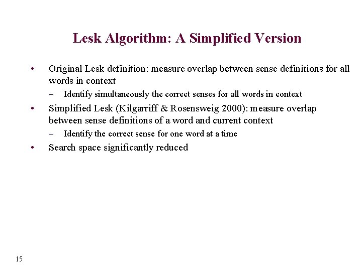
Lesk Algorithm: A Simplified Version • Original Lesk definition: measure overlap between sense definitions for all words in context – • Simplified Lesk (Kilgarriff & Rosensweig 2000): measure overlap between sense definitions of a word and current context – • 15 Identify simultaneously the correct senses for all words in context Identify the correct sense for one word at a time Search space significantly reduced

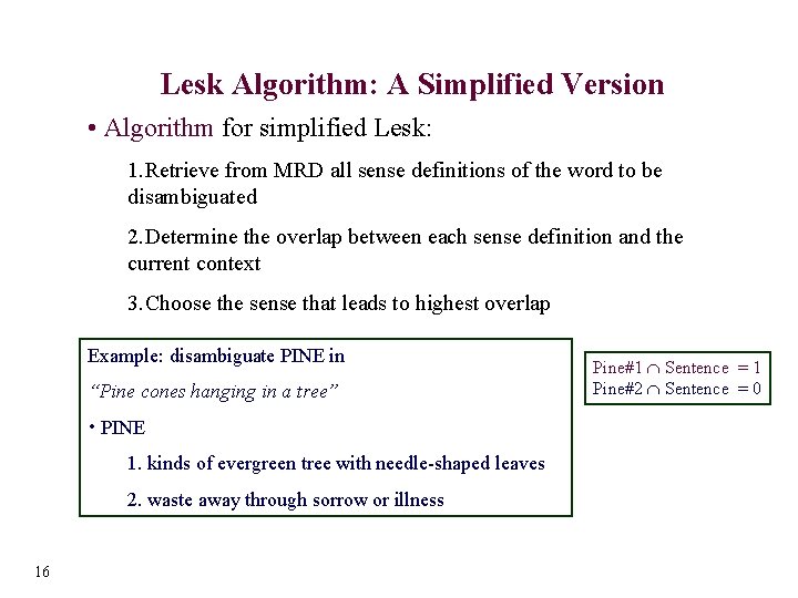
Lesk Algorithm: A Simplified Version • Algorithm for simplified Lesk: 1. Retrieve from MRD all sense definitions of the word to be disambiguated 2. Determine the overlap between each sense definition and the current context 3. Choose the sense that leads to highest overlap Example: disambiguate PINE in “Pine cones hanging in a tree” • PINE 1. kinds of evergreen tree with needle-shaped leaves 2. waste away through sorrow or illness 16 Pine#1 Sentence = 1 Pine#2 Sentence = 0

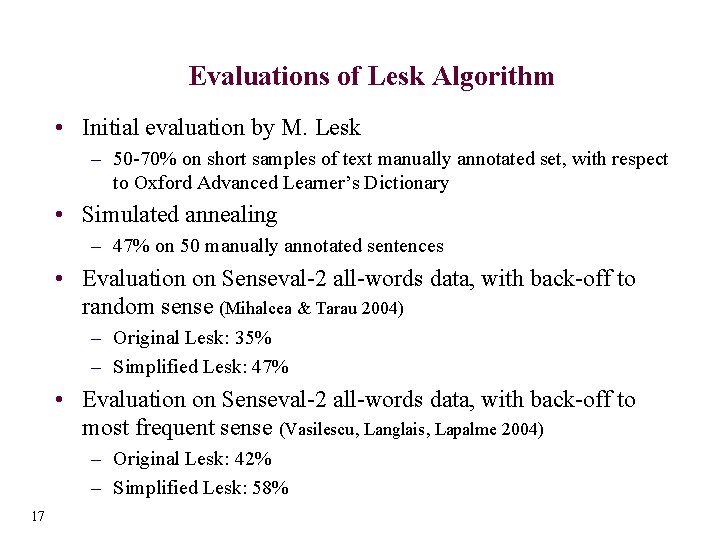
Evaluations of Lesk Algorithm • Initial evaluation by M. Lesk – 50 -70% on short samples of text manually annotated set, with respect to Oxford Advanced Learner’s Dictionary • Simulated annealing – 47% on 50 manually annotated sentences • Evaluation on Senseval-2 all-words data, with back-off to random sense (Mihalcea & Tarau 2004) – Original Lesk: 35% – Simplified Lesk: 47% • Evaluation on Senseval-2 all-words data, with back-off to most frequent sense (Vasilescu, Langlais, Lapalme 2004) – Original Lesk: 42% – Simplified Lesk: 58% 17

Outline • Task definition – Machine Readable Dictionaries • • 18 Algorithms based on Machine Readable Dictionaries Selectional Preferences Measures of Semantic Similarity Heuristic-based Methods

Unsupervised Disambiguation • Disambiguate word senses: – without supporting tools such as dictionaries and thesauri – without a labeled training text • Without such resources, word senses are not labeled – We cannot say “chair/furniture” or “chair/person” • We can: – Cluster/group the contexts of an ambiguous word into a number of groups – Discriminate between these groups without actually labeling them 19

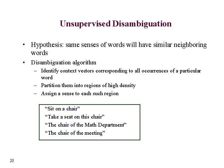
Unsupervised Disambiguation • Hypothesis: same senses of words will have similar neighboring words • Disambiguation algorithm – Identify context vectors corresponding to all occurrences of a particular word – Partition them into regions of high density – Assign a sense to each such region “Sit on a chair” “Take a seat on this chair” “The chair of the Math Department” “The chair of the meeting” 20

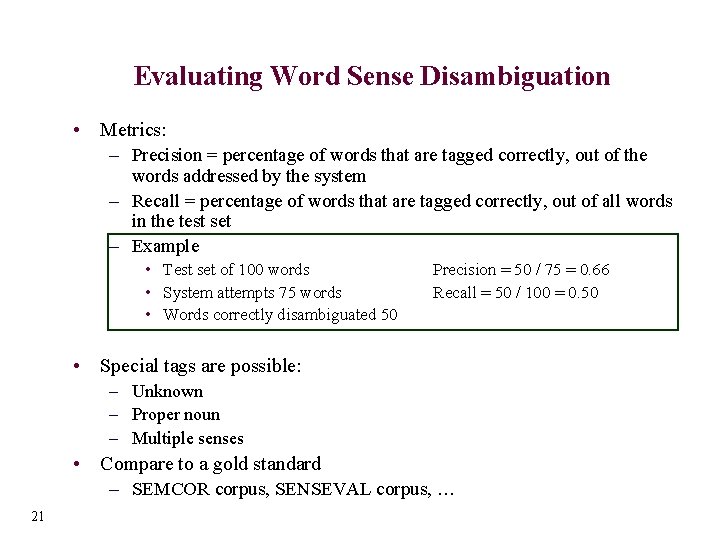
Evaluating Word Sense Disambiguation • Metrics: – Precision = percentage of words that are tagged correctly, out of the words addressed by the system – Recall = percentage of words that are tagged correctly, out of all words in the test set – Example • Test set of 100 words • System attempts 75 words • Words correctly disambiguated 50 Precision = 50 / 75 = 0. 66 Recall = 50 / 100 = 0. 50 • Special tags are possible: – Unknown – Proper noun – Multiple senses • Compare to a gold standard – SEMCOR corpus, SENSEVAL corpus, … 21

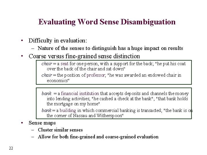
Evaluating Word Sense Disambiguation • Difficulty in evaluation: – Nature of the senses to distinguish has a huge impact on results • Coarse versus fine-grained sense distinction chair = a seat for one person, with a support for the back; "he put his coat over the back of the chair and sat down“ chair = the position of professor; "he was awarded an endowed chair in economics“ bank = a financial institution that accepts deposits and channels the money into lending activities; "he cashed a check at the bank"; "that bank holds the mortgage on my home" bank = a building in which commercial banking is transacted; "the bank is on the corner of Nassau and Witherspoon“ • Sense maps – Cluster similar senses – Allow for both fine-grained and coarse-grained evaluation 22

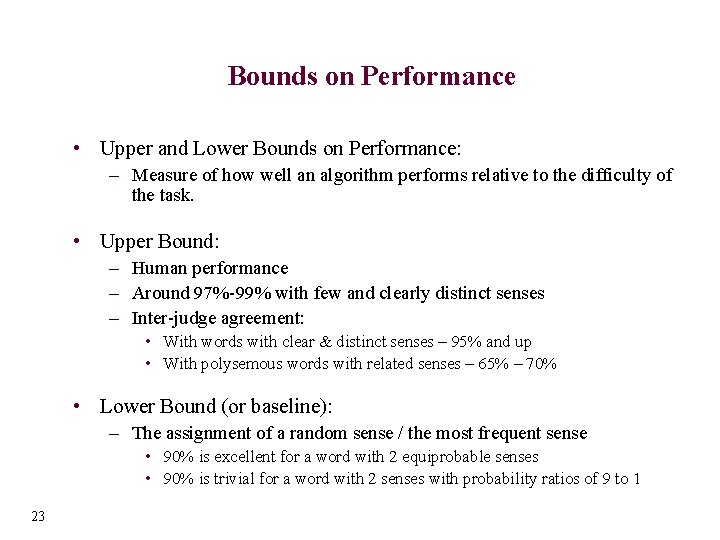
Bounds on Performance • Upper and Lower Bounds on Performance: – Measure of how well an algorithm performs relative to the difficulty of the task. • Upper Bound: – Human performance – Around 97%-99% with few and clearly distinct senses – Inter-judge agreement: • With words with clear & distinct senses – 95% and up • With polysemous words with related senses – 65% – 70% • Lower Bound (or baseline): – The assignment of a random sense / the most frequent sense • 90% is excellent for a word with 2 equiprobable senses • 90% is trivial for a word with 2 senses with probability ratios of 9 to 1 23

References • • 24 (Gale, Church and Yarowsky 1992) Gale, W. , Church, K. , and Yarowsky, D. Estimating upper and lower bounds on the performance of word-sense disambiguation programs ACL 1992. (Miller et. al. , 1994) Miller, G. , Chodorow, M. , Landes, S. , Leacock, C. , and Thomas, R. Using a semantic concordance for sense identification. ARPA Workshop 1994. (Miller, 1995) Miller, G. Wordnet: A lexical database. ACM, 38(11) 1995. (Senseval) Sensevaluation exercises http: //www. senseval. org

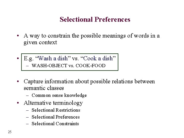
Selectional Preferences • A way to constrain the possible meanings of words in a given context • E. g. “Wash a dish” vs. “Cook a dish” – WASH-OBJECT vs. COOK-FOOD • Capture information about possible relations between semantic classes – Common sense knowledge • Alternative terminology – Selectional Restrictions – Selectional Preferences – Selectional Constraints 25

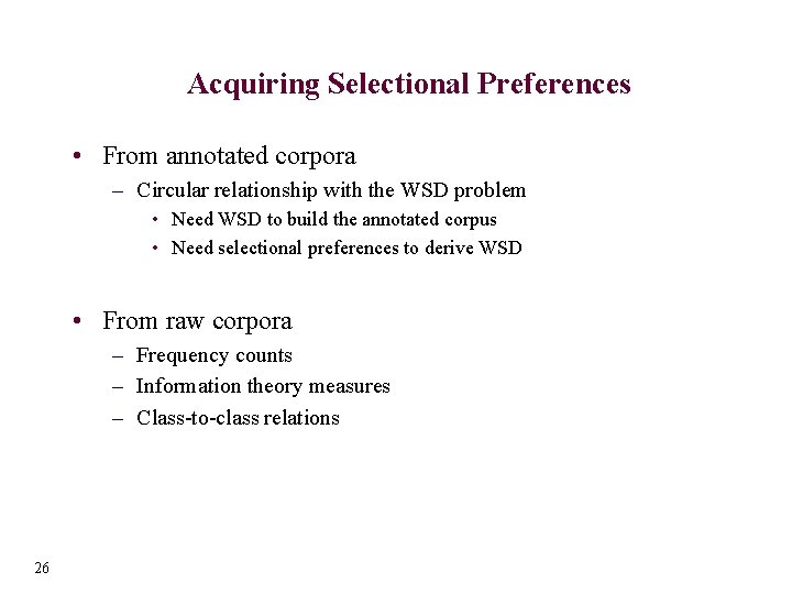
Acquiring Selectional Preferences • From annotated corpora – Circular relationship with the WSD problem • Need WSD to build the annotated corpus • Need selectional preferences to derive WSD • From raw corpora – Frequency counts – Information theory measures – Class-to-class relations 26

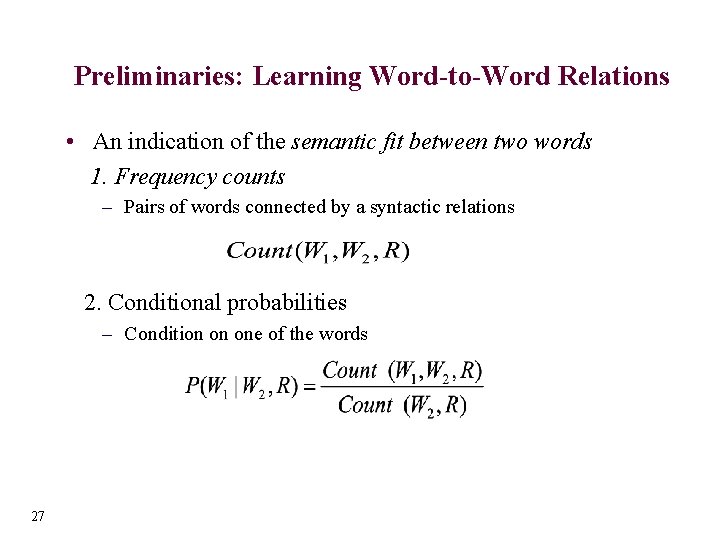
Preliminaries: Learning Word-to-Word Relations • An indication of the semantic fit between two words 1. Frequency counts – Pairs of words connected by a syntactic relations 2. Conditional probabilities – Condition on one of the words 27

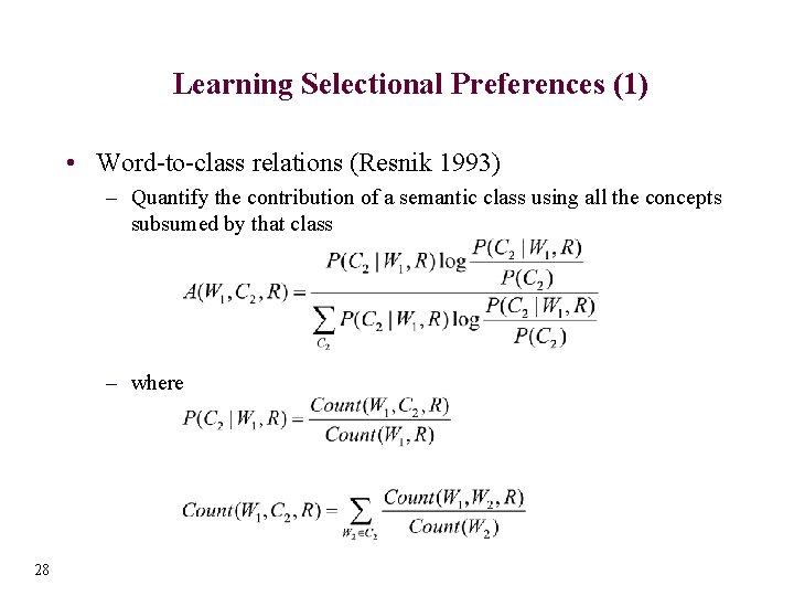
Learning Selectional Preferences (1) • Word-to-class relations (Resnik 1993) – Quantify the contribution of a semantic class using all the concepts subsumed by that class – where 28

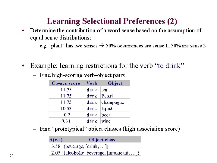
Learning Selectional Preferences (2) • Determine the contribution of a word sense based on the assumption of equal sense distributions: – e. g. “plant” has two senses 50% occurrences are sense 1, 50% are sense 2 • Example: learning restrictions for the verb “to drink” – Find high-scoring verb-object pairs – Find “prototypical” object classes (high association score) 29

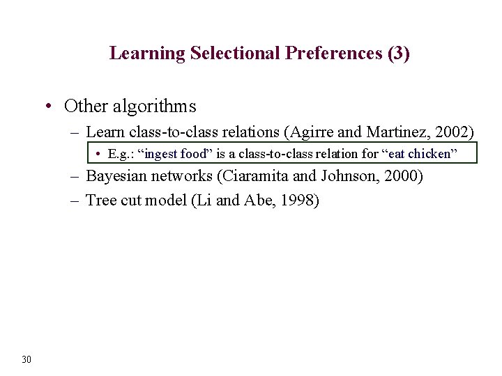
Learning Selectional Preferences (3) • Other algorithms – Learn class-to-class relations (Agirre and Martinez, 2002) • E. g. : “ingest food” is a class-to-class relation for “eat chicken” – Bayesian networks (Ciaramita and Johnson, 2000) – Tree cut model (Li and Abe, 1998) 30

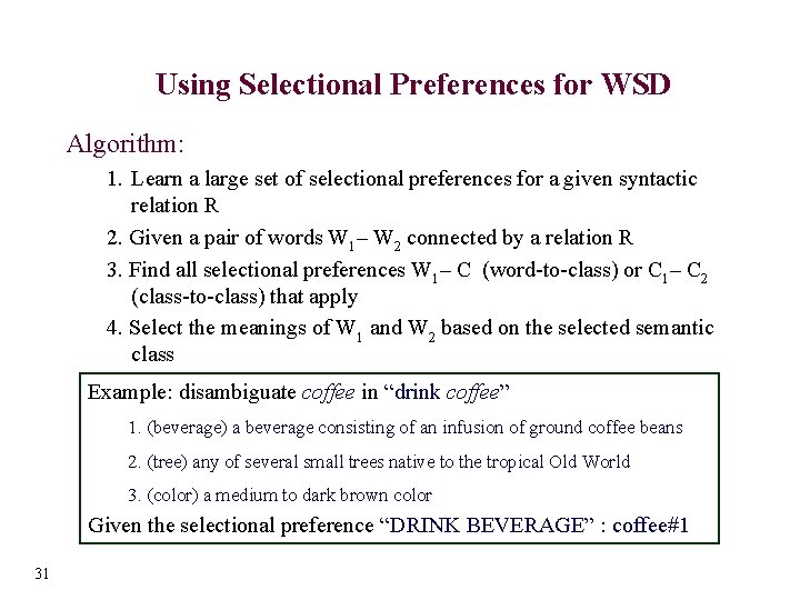
Using Selectional Preferences for WSD Algorithm: 1. Learn a large set of selectional preferences for a given syntactic relation R 2. Given a pair of words W 1– W 2 connected by a relation R 3. Find all selectional preferences W 1– C (word-to-class) or C 1– C 2 (class-to-class) that apply 4. Select the meanings of W 1 and W 2 based on the selected semantic class Example: disambiguate coffee in “drink coffee” 1. (beverage) a beverage consisting of an infusion of ground coffee beans 2. (tree) any of several small trees native to the tropical Old World 3. (color) a medium to dark brown color Given the selectional preference “DRINK BEVERAGE” : coffee#1 31

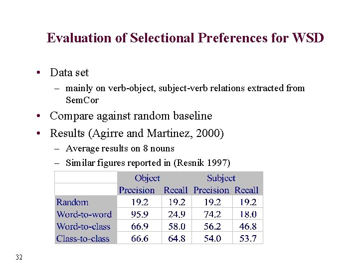
Evaluation of Selectional Preferences for WSD • Data set – mainly on verb-object, subject-verb relations extracted from Sem. Cor • Compare against random baseline • Results (Agirre and Martinez, 2000) – Average results on 8 nouns – Similar figures reported in (Resnik 1997) 32

Outline • Task definition – Machine Readable Dictionaries • • 33 Algorithms based on Machine Readable Dictionaries Selectional Restrictions Measures of Semantic Similarity Heuristic-based Methods

Semantic Similarity • Words in a discourse must be related in meaning, for the discourse to be coherent (Haliday and Hassan, 1976) • Use this property for WSD – Identify related meanings for words that share a common context • Context span: 1. Local context: semantic similarity between pairs of words 2. Global context: lexical chains 34

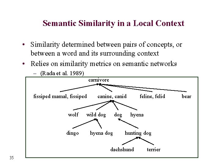
Semantic Similarity in a Local Context • Similarity determined between pairs of concepts, or between a word and its surrounding context • Relies on similarity metrics on semantic networks – (Rada et al. 1989) carnivore fissiped mamal, fissiped wolf dingo canine, canid wild dog hyena dog feline, felid hyena hunting dog dachshund 35 terrier bear

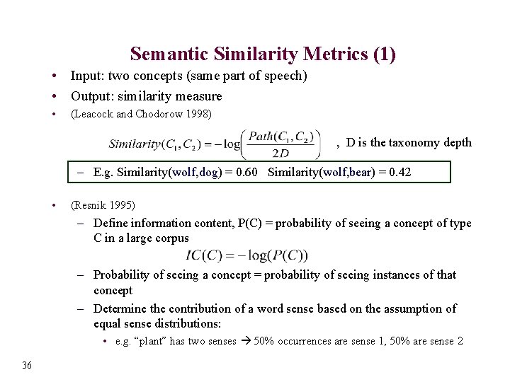
Semantic Similarity Metrics (1) • Input: two concepts (same part of speech) • Output: similarity measure • (Leacock and Chodorow 1998) , D is the taxonomy depth – E. g. Similarity(wolf, dog) = 0. 60 Similarity(wolf, bear) = 0. 42 • (Resnik 1995) – Define information content, P(C) = probability of seeing a concept of type C in a large corpus – Probability of seeing a concept = probability of seeing instances of that concept – Determine the contribution of a word sense based on the assumption of equal sense distributions: • e. g. “plant” has two senses 50% occurrences are sense 1, 50% are sense 2 36

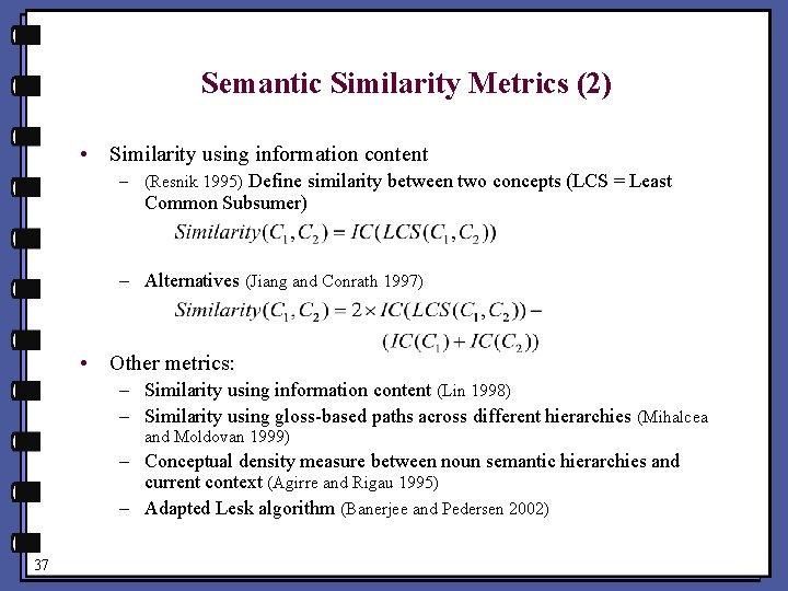
Semantic Similarity Metrics (2) • Similarity using information content – (Resnik 1995) Define similarity between two concepts (LCS = Least Common Subsumer) – Alternatives (Jiang and Conrath 1997) • Other metrics: – Similarity using information content (Lin 1998) – Similarity using gloss-based paths across different hierarchies (Mihalcea and Moldovan 1999) – Conceptual density measure between noun semantic hierarchies and current context (Agirre and Rigau 1995) – Adapted Lesk algorithm (Banerjee and Pedersen 2002) 37

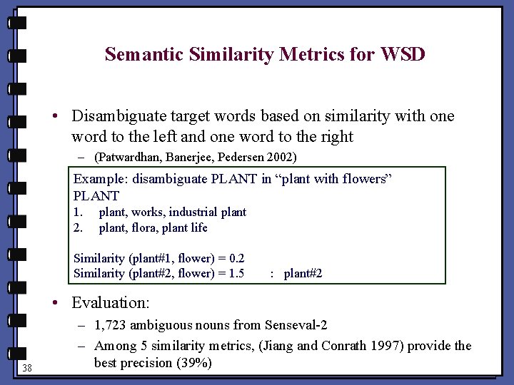
Semantic Similarity Metrics for WSD • Disambiguate target words based on similarity with one word to the left and one word to the right – (Patwardhan, Banerjee, Pedersen 2002) Example: disambiguate PLANT in “plant with flowers” PLANT 1. 2. plant, works, industrial plant, flora, plant life Similarity (plant#1, flower) = 0. 2 Similarity (plant#2, flower) = 1. 5 : plant#2 • Evaluation: 38 – 1, 723 ambiguous nouns from Senseval-2 – Among 5 similarity metrics, (Jiang and Conrath 1997) provide the best precision (39%)

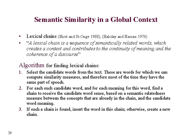
Semantic Similarity in a Global Context • • Lexical chains (Hirst and St-Onge 1988), (Haliday and Hassan 1976) “A lexical chain is a sequence of semantically related words, which creates a context and contributes to the continuity of meaning and the coherence of a discourse” Algorithm for finding lexical chains: 1. Select the candidate words from the text. These are words for which we can compute similarity measures, and therefore most of the time they have the same part of speech. 2. For each such candidate word, and for each meaning for this word, find a chain to receive the candidate word sense, based on a semantic relatedness measure between the concepts that are already in the chain, and the candidate word meaning. 3. If such a chain is found, insert the word in this chain; otherwise, create a new chain. 39

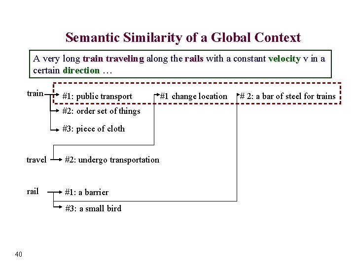
Semantic Similarity of a Global Context A very long train traveling along the rails with a constant velocity v in a certain direction … train #1: public transport #2: order set of things #3: piece of cloth travel #2: undergo transportation rail #1: a barrier #3: a small bird 40 #1 change location # 2: a bar of steel for trains

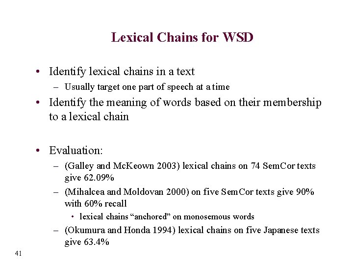
Lexical Chains for WSD • Identify lexical chains in a text – Usually target one part of speech at a time • Identify the meaning of words based on their membership to a lexical chain • Evaluation: – (Galley and Mc. Keown 2003) lexical chains on 74 Sem. Cor texts give 62. 09% – (Mihalcea and Moldovan 2000) on five Sem. Cor texts give 90% with 60% recall • lexical chains “anchored” on monosemous words – (Okumura and Honda 1994) lexical chains on five Japanese texts give 63. 4% 41

Outline • Task definition – Machine Readable Dictionaries • • 42 Algorithms based on Machine Readable Dictionaries Selectional Restrictions Measures of Semantic Similarity Heuristic-based Methods

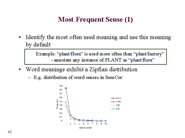
Most Frequent Sense (1) • Identify the most often used meaning and use this meaning by default Example: “plant/flora” is used more often than “plant/factory” - annotate any instance of PLANT as “plant/flora” • Word meanings exhibit a Zipfian distribution – E. g. distribution of word senses in Sem. Cor 43

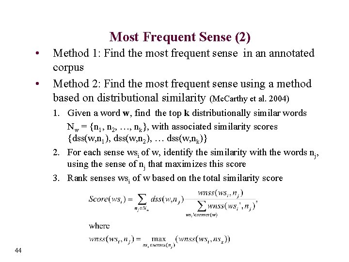
Most Frequent Sense (2) • • Method 1: Find the most frequent sense in an annotated corpus Method 2: Find the most frequent sense using a method based on distributional similarity (Mc. Carthy et al. 2004) 1. Given a word w, find the top k distributionally similar words Nw = {n 1, n 2, …, nk}, with associated similarity scores {dss(w, n 1), dss(w, n 2), … dss(w, nk)} 2. For each sense wsi of w, identify the similarity with the words nj, using the sense of nj that maximizes this score 3. Rank senses wsi of w based on the total similarity score 44

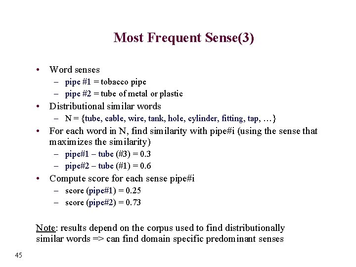
Most Frequent Sense(3) • Word senses – pipe #1 = tobacco pipe – pipe #2 = tube of metal or plastic • Distributional similar words – N = {tube, cable, wire, tank, hole, cylinder, fitting, tap, …} • For each word in N, find similarity with pipe#i (using the sense that maximizes the similarity) – pipe#1 – tube (#3) = 0. 3 – pipe#2 – tube (#1) = 0. 6 • Compute score for each sense pipe#i – score (pipe#1) = 0. 25 – score (pipe#2) = 0. 73 Note: results depend on the corpus used to find distributionally similar words => can find domain specific predominant senses 45

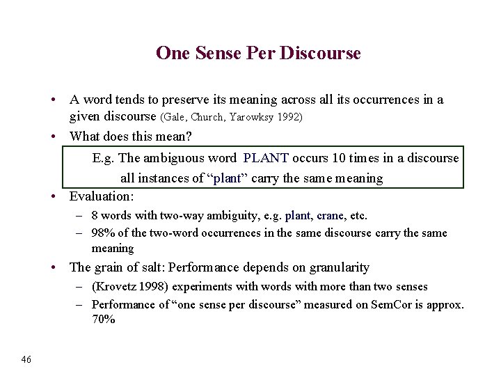
One Sense Per Discourse • A word tends to preserve its meaning across all its occurrences in a given discourse (Gale, Church, Yarowksy 1992) • What does this mean? E. g. The ambiguous word PLANT occurs 10 times in a discourse all instances of “plant” carry the same meaning • Evaluation: – 8 words with two-way ambiguity, e. g. plant, crane, etc. – 98% of the two-word occurrences in the same discourse carry the same meaning • The grain of salt: Performance depends on granularity – (Krovetz 1998) experiments with words with more than two senses – Performance of “one sense per discourse” measured on Sem. Cor is approx. 70% 46

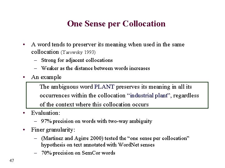
One Sense per Collocation • A word tends to preserver its meaning when used in the same collocation (Yarowsky 1993) – Strong for adjacent collocations – Weaker as the distance between words increases • An example The ambiguous word PLANT preserves its meaning in all its occurrences within the collocation “industrial plant”, regardless of the context where this collocation occurs • Evaluation: – 97% precision on words with two-way ambiguity • Finer granularity: – (Martinez and Agirre 2000) tested the “one sense per collocation” hypothesis on text annotated with Word. Net senses – 70% precision on Sem. Cor words 47

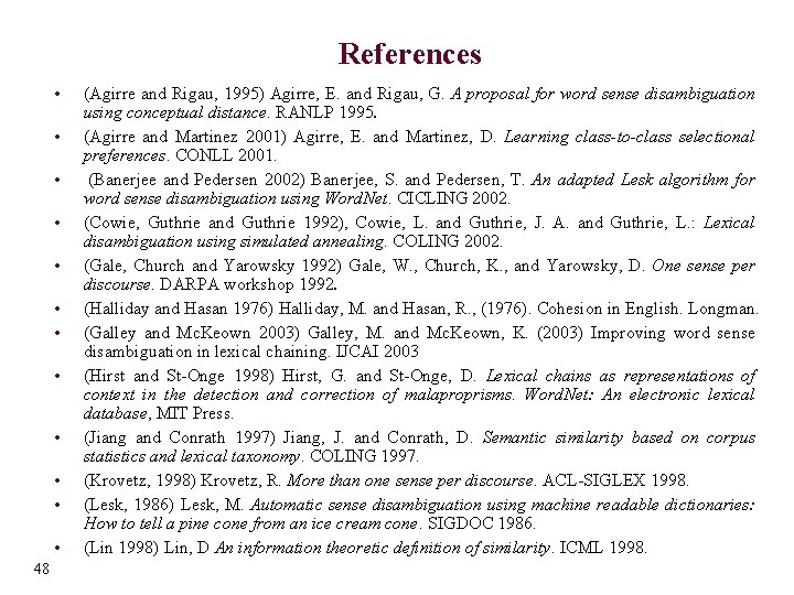
References • • • 48 (Agirre and Rigau, 1995) Agirre, E. and Rigau, G. A proposal for word sense disambiguation using conceptual distance. RANLP 1995. (Agirre and Martinez 2001) Agirre, E. and Martinez, D. Learning class-to-class selectional preferences. CONLL 2001. (Banerjee and Pedersen 2002) Banerjee, S. and Pedersen, T. An adapted Lesk algorithm for word sense disambiguation using Word. Net. CICLING 2002. (Cowie, Guthrie and Guthrie 1992), Cowie, L. and Guthrie, J. A. and Guthrie, L. : Lexical disambiguation using simulated annealing. COLING 2002. (Gale, Church and Yarowsky 1992) Gale, W. , Church, K. , and Yarowsky, D. One sense per discourse. DARPA workshop 1992. (Halliday and Hasan 1976) Halliday, M. and Hasan, R. , (1976). Cohesion in English. Longman. (Galley and Mc. Keown 2003) Galley, M. and Mc. Keown, K. (2003) Improving word sense disambiguation in lexical chaining. IJCAI 2003 (Hirst and St-Onge 1998) Hirst, G. and St-Onge, D. Lexical chains as representations of context in the detection and correction of malaproprisms. Word. Net: An electronic lexical database, MIT Press. (Jiang and Conrath 1997) Jiang, J. and Conrath, D. Semantic similarity based on corpus statistics and lexical taxonomy. COLING 1997. (Krovetz, 1998) Krovetz, R. More than one sense per discourse. ACL-SIGLEX 1998. (Lesk, 1986) Lesk, M. Automatic sense disambiguation using machine readable dictionaries: How to tell a pine cone from an ice cream cone. SIGDOC 1986. (Lin 1998) Lin, D An information theoretic definition of similarity. ICML 1998.

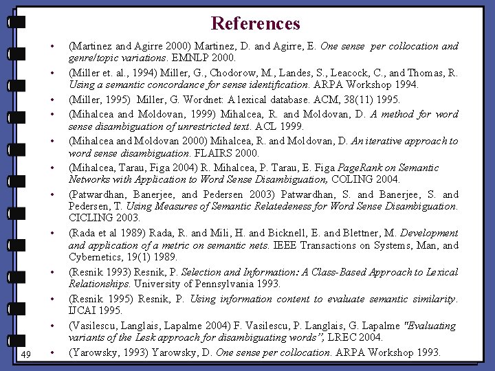
References • • • 49 • (Martinez and Agirre 2000) Martinez, D. and Agirre, E. One sense per collocation and genre/topic variations. EMNLP 2000. (Miller et. al. , 1994) Miller, G. , Chodorow, M. , Landes, S. , Leacock, C. , and Thomas, R. Using a semantic concordance for sense identification. ARPA Workshop 1994. (Miller, 1995) Miller, G. Wordnet: A lexical database. ACM, 38(11) 1995. (Mihalcea and Moldovan, 1999) Mihalcea, R. and Moldovan, D. A method for word sense disambiguation of unrestricted text. ACL 1999. (Mihalcea and Moldovan 2000) Mihalcea, R. and Moldovan, D. An iterative approach to word sense disambiguation. FLAIRS 2000. (Mihalcea, Tarau, Figa 2004) R. Mihalcea, P. Tarau, E. Figa Page. Rank on Semantic Networks with Application to Word Sense Disambiguation, COLING 2004. (Patwardhan, Banerjee, and Pedersen 2003) Patwardhan, S. and Banerjee, S. and Pedersen, T. Using Measures of Semantic Relatedeness for Word Sense Disambiguation. CICLING 2003. (Rada et al 1989) Rada, R. and Mili, H. and Bicknell, E. and Blettner, M. Development and application of a metric on semantic nets. IEEE Transactions on Systems, Man, and Cybernetics, 19(1) 1989. (Resnik 1993) Resnik, P. Selection and Information: A Class-Based Approach to Lexical Relationships. University of Pennsylvania 1993. (Resnik 1995) Resnik, P. Using information content to evaluate semantic similarity. IJCAI 1995. (Vasilescu, Langlais, Lapalme 2004) F. Vasilescu, P. Langlais, G. Lapalme "Evaluating variants of the Lesk approach for disambiguating words”, LREC 2004. (Yarowsky, 1993) Yarowsky, D. One sense per collocation. ARPA Workshop 1993.

Part 4: Supervised Methods of Word Sense Disambiguation

Outline • What is Supervised Learning? • Task Definition • Single Classifiers – Naïve Bayesian Classifiers – Decision Lists and Trees • Ensembles of Classifiers 51

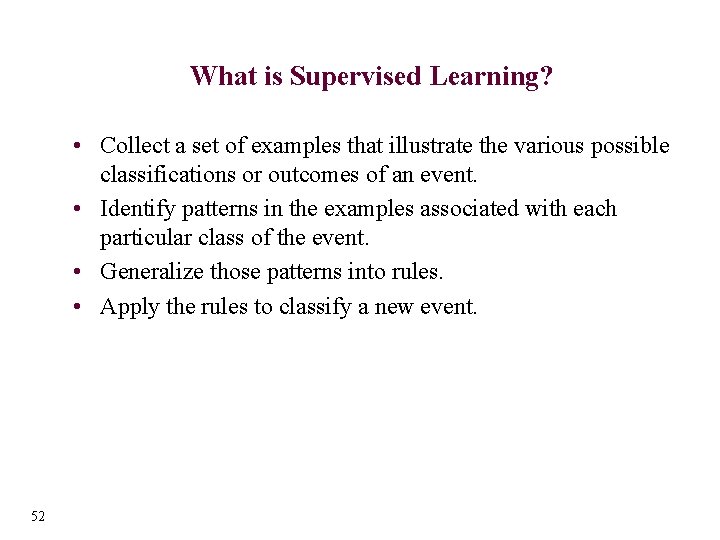
What is Supervised Learning? • Collect a set of examples that illustrate the various possible classifications or outcomes of an event. • Identify patterns in the examples associated with each particular class of the event. • Generalize those patterns into rules. • Apply the rules to classify a new event. 52

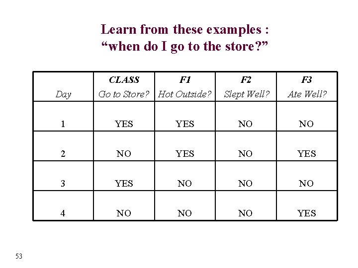
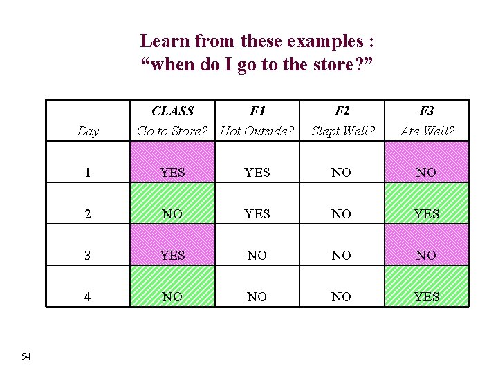
Learn from these examples : “when do I go to the store? ” Day 53 CLASS F 1 Go to Store? Hot Outside? F 2 Slept Well? F 3 Ate Well? 1 YES NO NO 2 NO YES 3 YES NO NO NO 4 NO NO NO YES

Learn from these examples : “when do I go to the store? ” Day 54 CLASS F 1 Go to Store? Hot Outside? F 2 Slept Well? F 3 Ate Well? 1 YES NO NO 2 NO YES 3 YES NO NO NO 4 NO NO NO YES

Outline • What is Supervised Learning? • Task Definition • Single Classifiers – Naïve Bayesian Classifiers – Decision Lists and Trees • Ensembles of Classifiers 55

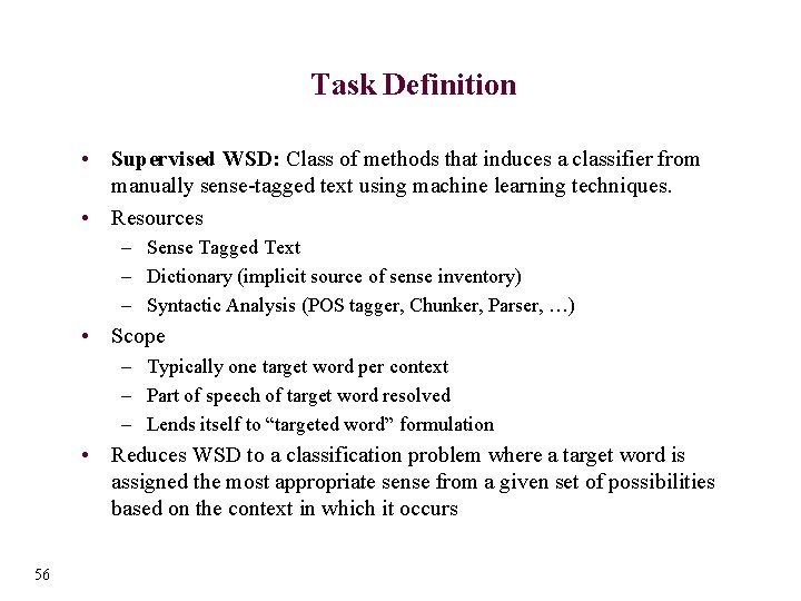
Task Definition • Supervised WSD: Class of methods that induces a classifier from manually sense-tagged text using machine learning techniques. • Resources – Sense Tagged Text – Dictionary (implicit source of sense inventory) – Syntactic Analysis (POS tagger, Chunker, Parser, …) • Scope – Typically one target word per context – Part of speech of target word resolved – Lends itself to “targeted word” formulation • Reduces WSD to a classification problem where a target word is assigned the most appropriate sense from a given set of possibilities based on the context in which it occurs 56

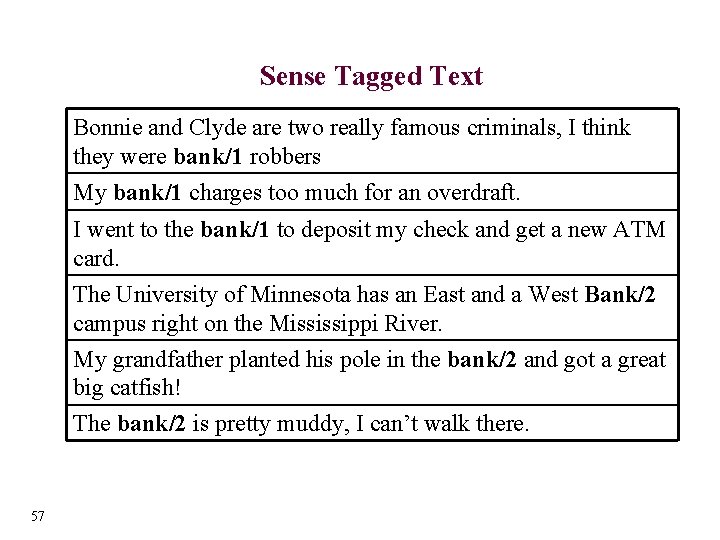
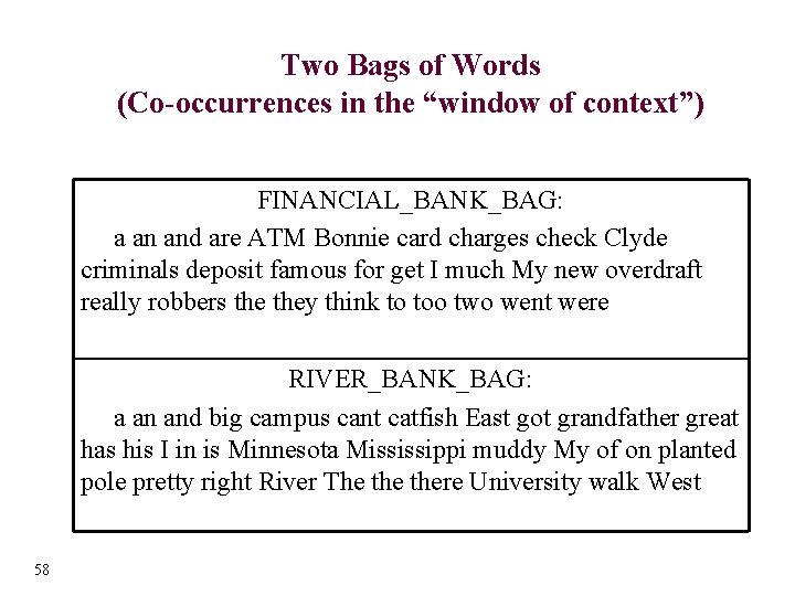
Sense Tagged Text Bonnie and Clyde are two really famous criminals, I think they were bank/1 robbers My bank/1 charges too much for an overdraft. I went to the bank/1 to deposit my check and get a new ATM card. The University of Minnesota has an East and a West Bank/2 campus right on the Mississippi River. My grandfather planted his pole in the bank/2 and got a great big catfish! The bank/2 is pretty muddy, I can’t walk there. 57

Two Bags of Words (Co-occurrences in the “window of context”) FINANCIAL_BANK_BAG: a an and are ATM Bonnie card charges check Clyde criminals deposit famous for get I much My new overdraft really robbers they think to too two went were RIVER_BANK_BAG: a an and big campus cant catfish East got grandfather great has his I in is Minnesota Mississippi muddy My of on planted pole pretty right River The there University walk West 58

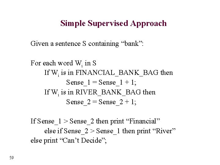
Simple Supervised Approach Given a sentence S containing “bank”: For each word Wi in S If Wi is in FINANCIAL_BANK_BAG then Sense_1 = Sense_1 + 1; If Wi is in RIVER_BANK_BAG then Sense_2 = Sense_2 + 1; If Sense_1 > Sense_2 then print “Financial” else if Sense_2 > Sense_1 then print “River” else print “Can’t Decide”; 59

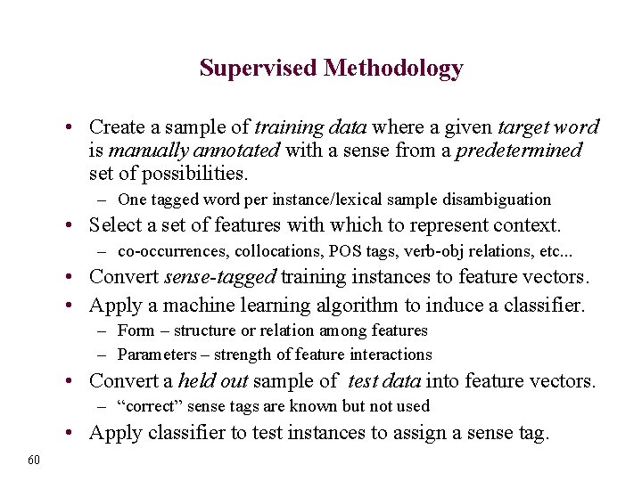
Supervised Methodology • Create a sample of training data where a given target word is manually annotated with a sense from a predetermined set of possibilities. – One tagged word per instance/lexical sample disambiguation • Select a set of features with which to represent context. – co-occurrences, collocations, POS tags, verb-obj relations, etc. . . • Convert sense-tagged training instances to feature vectors. • Apply a machine learning algorithm to induce a classifier. – Form – structure or relation among features – Parameters – strength of feature interactions • Convert a held out sample of test data into feature vectors. – “correct” sense tags are known but not used • Apply classifier to test instances to assign a sense tag. 60

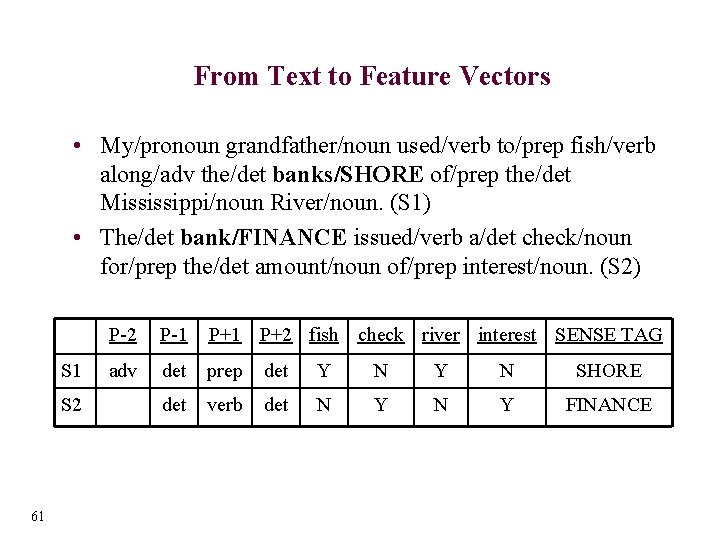
From Text to Feature Vectors • My/pronoun grandfather/noun used/verb to/prep fish/verb along/adv the/det banks/SHORE of/prep the/det Mississippi/noun River/noun. (S 1) • The/det bank/FINANCE issued/verb a/det check/noun for/prep the/det amount/noun of/prep interest/noun. (S 2) S 1 S 2 61 P-2 P-1 P+2 fish check river interest SENSE TAG adv det prep det Y N SHORE det verb det N Y FINANCE

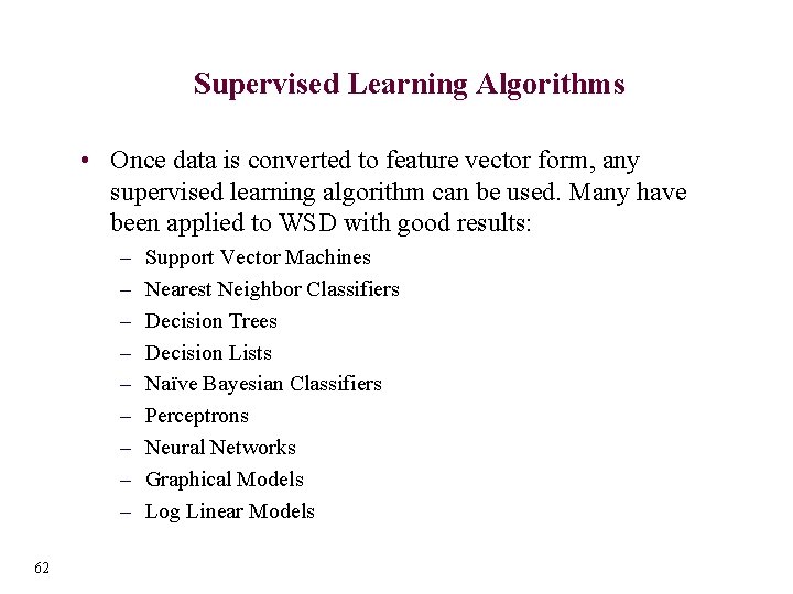
Supervised Learning Algorithms • Once data is converted to feature vector form, any supervised learning algorithm can be used. Many have been applied to WSD with good results: – – – – – 62 Support Vector Machines Nearest Neighbor Classifiers Decision Trees Decision Lists Naïve Bayesian Classifiers Perceptrons Neural Networks Graphical Models Log Linear Models

Outline • • • 63 What is Supervised Learning? Task Definition Naïve Bayesian Classifier Decision Lists and Trees Ensembles of Classifiers

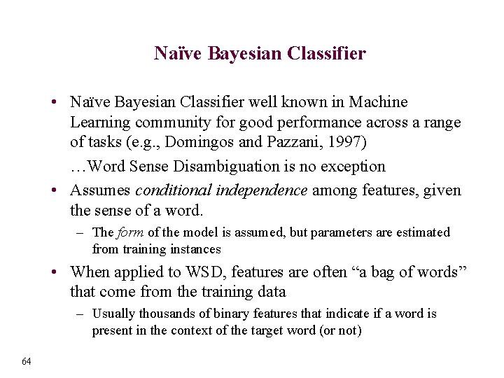
Naïve Bayesian Classifier • Naïve Bayesian Classifier well known in Machine Learning community for good performance across a range of tasks (e. g. , Domingos and Pazzani, 1997) …Word Sense Disambiguation is no exception • Assumes conditional independence among features, given the sense of a word. – The form of the model is assumed, but parameters are estimated from training instances • When applied to WSD, features are often “a bag of words” that come from the training data – Usually thousands of binary features that indicate if a word is present in the context of the target word (or not) 64

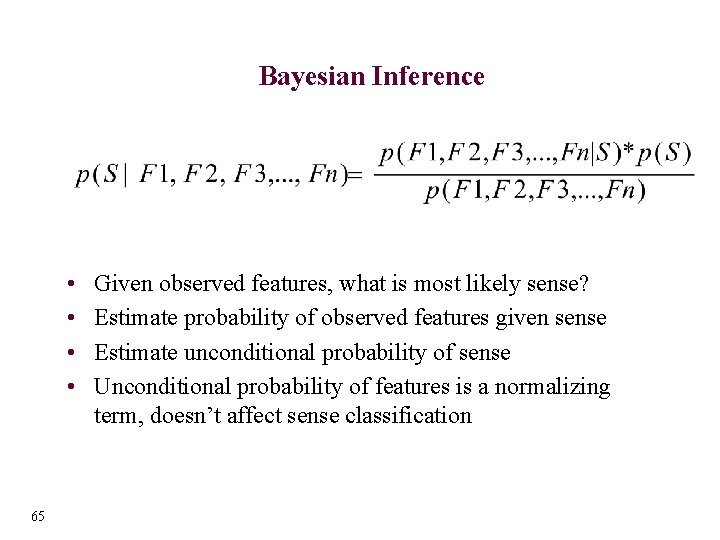
Bayesian Inference • • 65 Given observed features, what is most likely sense? Estimate probability of observed features given sense Estimate unconditional probability of sense Unconditional probability of features is a normalizing term, doesn’t affect sense classification

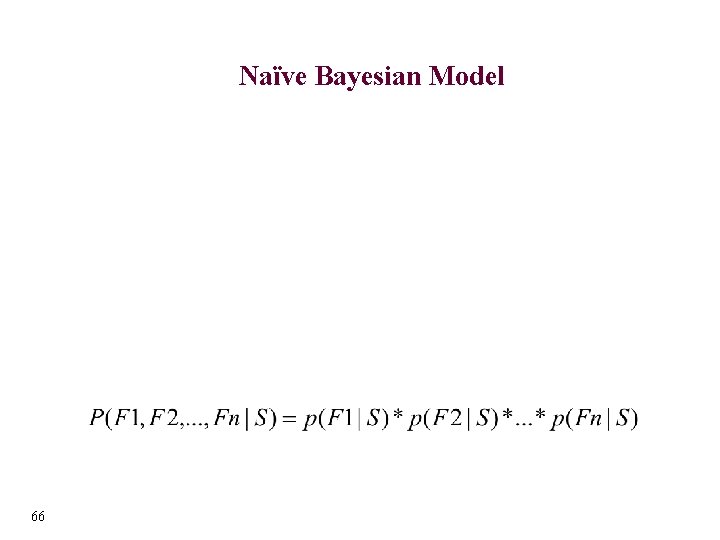
Naïve Bayesian Model 66

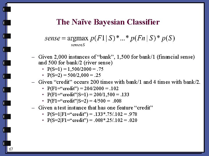
The Naïve Bayesian Classifier – Given 2, 000 instances of “bank”, 1, 500 for bank/1 (financial sense) and 500 for bank/2 (river sense) • P(S=1) = 1, 500/2000 =. 75 • P(S=2) = 500/2, 000 =. 25 – Given “credit” occurs 200 times with bank/1 and 4 times with bank/2. • P(F 1=“credit”) = 204/2000 =. 102 • P(F 1=“credit”|S=1) = 200/1, 500 =. 133 • P(F 1=“credit”|S=2) = 4/500 = . 008 – Given a test instance that has one feature “credit” • P(S=1|F 1=“credit”) =. 133*. 75/. 102 =. 978 • P(S=2|F 1=“credit”) =. 008*. 25/. 102 =. 020 67

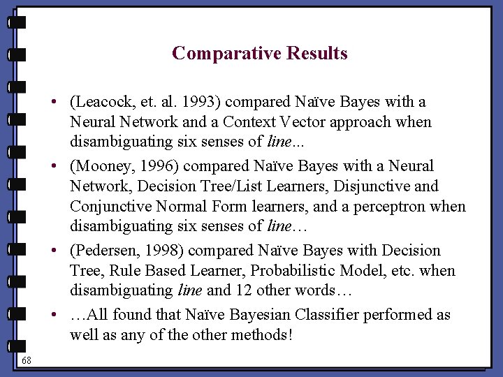
Comparative Results • (Leacock, et. al. 1993) compared Naïve Bayes with a Neural Network and a Context Vector approach when disambiguating six senses of line… • (Mooney, 1996) compared Naïve Bayes with a Neural Network, Decision Tree/List Learners, Disjunctive and Conjunctive Normal Form learners, and a perceptron when disambiguating six senses of line… • (Pedersen, 1998) compared Naïve Bayes with Decision Tree, Rule Based Learner, Probabilistic Model, etc. when disambiguating line and 12 other words… • …All found that Naïve Bayesian Classifier performed as well as any of the other methods! 68

Outline • • • 69 What is Supervised Learning? Task Definition Naïve Bayesian Classifiers Decision Lists and Trees Ensembles of Classifiers

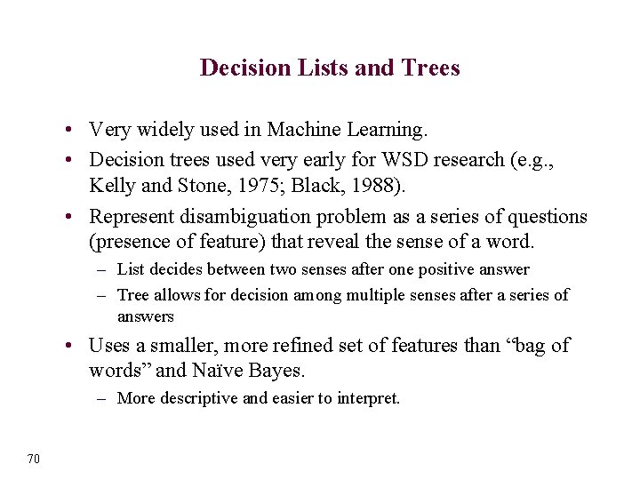
Decision Lists and Trees • Very widely used in Machine Learning. • Decision trees used very early for WSD research (e. g. , Kelly and Stone, 1975; Black, 1988). • Represent disambiguation problem as a series of questions (presence of feature) that reveal the sense of a word. – List decides between two senses after one positive answer – Tree allows for decision among multiple senses after a series of answers • Uses a smaller, more refined set of features than “bag of words” and Naïve Bayes. – More descriptive and easier to interpret. 70

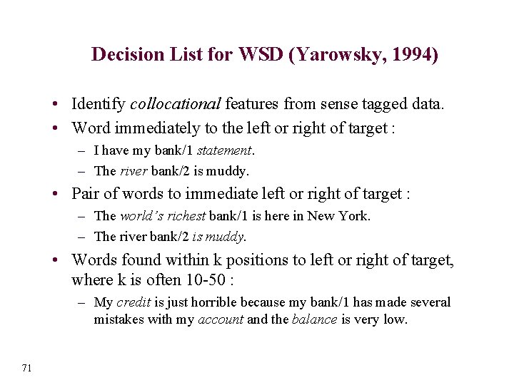
Decision List for WSD (Yarowsky, 1994) • Identify collocational features from sense tagged data. • Word immediately to the left or right of target : – I have my bank/1 statement. – The river bank/2 is muddy. • Pair of words to immediate left or right of target : – The world’s richest bank/1 is here in New York. – The river bank/2 is muddy. • Words found within k positions to left or right of target, where k is often 10 -50 : – My credit is just horrible because my bank/1 has made several mistakes with my account and the balance is very low. 71

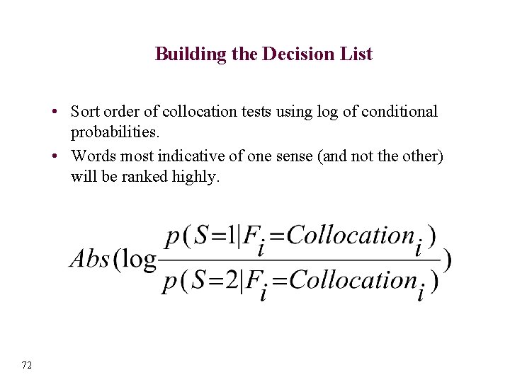
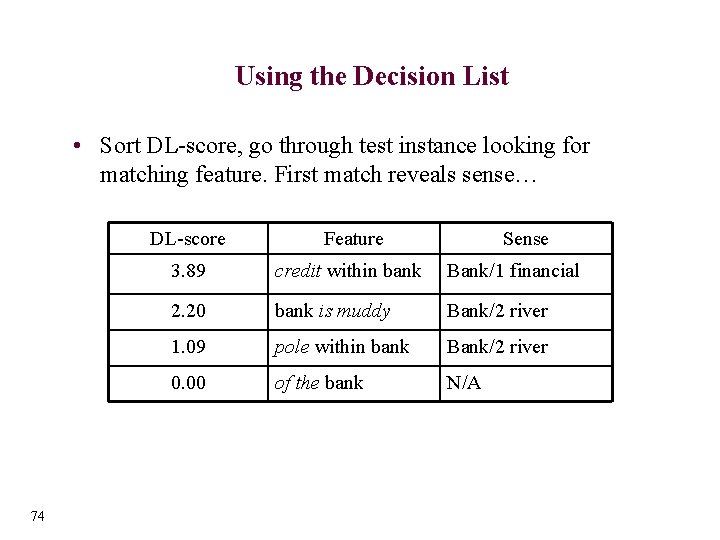
Building the Decision List • Sort order of collocation tests using log of conditional probabilities. • Words most indicative of one sense (and not the other) will be ranked highly. 72

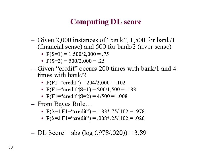
Computing DL score – Given 2, 000 instances of “bank”, 1, 500 for bank/1 (financial sense) and 500 for bank/2 (river sense) • P(S=1) = 1, 500/2, 000 =. 75 • P(S=2) = 500/2, 000 =. 25 – Given “credit” occurs 200 times with bank/1 and 4 times with bank/2. • P(F 1=“credit”) = 204/2, 000 =. 102 • P(F 1=“credit”|S=1) = 200/1, 500 =. 133 • P(F 1=“credit”|S=2) = 4/500 = . 008 – From Bayes Rule… • P(S=1|F 1=“credit”) =. 133*. 75/. 102 =. 978 • P(S=2|F 1=“credit”) =. 008*. 25/. 102 =. 020 – DL Score = abs (log (. 978/. 020)) = 3. 89 73

Using the Decision List • Sort DL-score, go through test instance looking for matching feature. First match reveals sense… 74 DL-score Feature Sense 3. 89 credit within bank Bank/1 financial 2. 20 bank is muddy Bank/2 river 1. 09 pole within bank Bank/2 river 0. 00 of the bank N/A

Using the Decision List 75

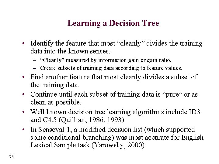
Learning a Decision Tree • Identify the feature that most “cleanly” divides the training data into the known senses. – “Cleanly” measured by information gain or gain ratio. – Create subsets of training data according to feature values. • Find another feature that most cleanly divides a subset of the training data. • Continue until each subset of training data is “pure” or as clean as possible. • Well known decision tree learning algorithms include ID 3 and C 4. 5 (Quillian, 1986, 1993) • In Senseval-1, a modified decision list (which supported some conditional branching) was most accurate for English Lexical Sample task (Yarowsky, 2000) 76

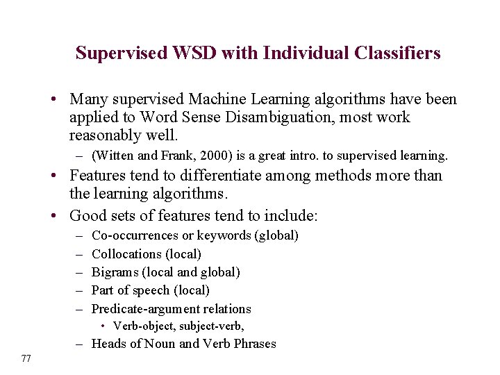
Supervised WSD with Individual Classifiers • Many supervised Machine Learning algorithms have been applied to Word Sense Disambiguation, most work reasonably well. – (Witten and Frank, 2000) is a great intro. to supervised learning. • Features tend to differentiate among methods more than the learning algorithms. • Good sets of features tend to include: – – – Co-occurrences or keywords (global) Collocations (local) Bigrams (local and global) Part of speech (local) Predicate-argument relations • Verb-object, subject-verb, – Heads of Noun and Verb Phrases 77

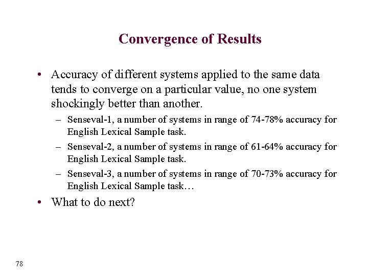
Convergence of Results • Accuracy of different systems applied to the same data tends to converge on a particular value, no one system shockingly better than another. – Senseval-1, a number of systems in range of 74 -78% accuracy for English Lexical Sample task. – Senseval-2, a number of systems in range of 61 -64% accuracy for English Lexical Sample task. – Senseval-3, a number of systems in range of 70 -73% accuracy for English Lexical Sample task… • What to do next? 78

Outline • • • 79 What is Supervised Learning? Task Definition Naïve Bayesian Classifiers Decision Lists and Trees Ensembles of Classifiers

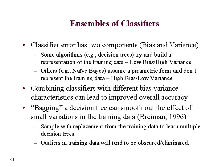
Ensembles of Classifiers • Classifier error has two components (Bias and Variance) – Some algorithms (e. g. , decision trees) try and build a representation of the training data – Low Bias/High Variance – Others (e. g. , Naïve Bayes) assume a parametric form and don’t represent the training data – High Bias/Low Variance • Combining classifiers with different bias variance characteristics can lead to improved overall accuracy • “Bagging” a decision tree can smooth out the effect of small variations in the training data (Breiman, 1996) – Sample with replacement from the training data to learn multiple decision trees. – Outliers in training data will tend to be obscured/eliminated. 80

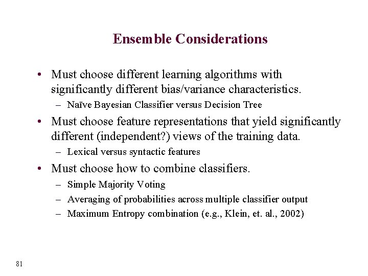
Ensemble Considerations • Must choose different learning algorithms with significantly different bias/variance characteristics. – Naïve Bayesian Classifier versus Decision Tree • Must choose feature representations that yield significantly different (independent? ) views of the training data. – Lexical versus syntactic features • Must choose how to combine classifiers. – Simple Majority Voting – Averaging of probabilities across multiple classifier output – Maximum Entropy combination (e. g. , Klein, et. al. , 2002) 81

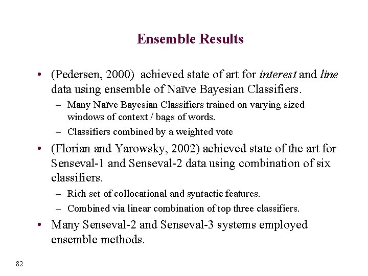
Ensemble Results • (Pedersen, 2000) achieved state of art for interest and line data using ensemble of Naïve Bayesian Classifiers. – Many Naïve Bayesian Classifiers trained on varying sized windows of context / bags of words. – Classifiers combined by a weighted vote • (Florian and Yarowsky, 2002) achieved state of the art for Senseval-1 and Senseval-2 data using combination of six classifiers. – Rich set of collocational and syntactic features. – Combined via linear combination of top three classifiers. • Many Senseval-2 and Senseval-3 systems employed ensemble methods. 82

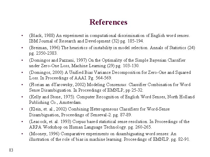
References • • • 83 (Black, 1988) An experiment in computational discrimination of English word senses. IBM Journal of Research and Development (32) pg. 185 -194. (Breiman, 1996) The heuristics of instability in model selection. Annals of Statistics (24) pg. 2350 -2383. (Domingos and Pazzani, 1997) On the Optimality of the Simple Bayesian Classifier under Zero-One Loss, Machine Learning (29) pg. 103 -130. (Domingos, 2000) A Unified Bias Variance Decomposition for Zero-One and Squared Loss. In Proceedings of AAAI. Pg. 564 -569. (Florian an d. Yarowsky, 2002) Modeling Consensus: Classifier Combination for Word Sense Disambiguation. In Proceedings of EMNLP, pp 25 -32. (Kelly and Stone, 1975). Computer Recognition of English Word Senses, North Holland Publishing Co. , Amsterdam. (Klein, et. al. , 2002) Combining Heterogeneous Classifiers for Word-Sense Disambiguation, Proceedings of Senseval-2. pg. 87 -89. (Leacock, et. al. 1993) Corpus based statistical sense resolution. In Proceedings of the ARPA Workshop on Human Language Technology. pg. 260 -265. (Mooney, 1996) Comparative experiments on disambiguating word senses: An illustration of the role of bias in machine learning. Proceedings of EMNLP. pg. 82 -91.

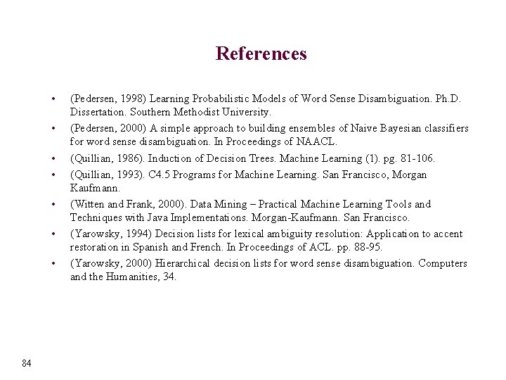
References • • 84 (Pedersen, 1998) Learning Probabilistic Models of Word Sense Disambiguation. Ph. D. Dissertation. Southern Methodist University. (Pedersen, 2000) A simple approach to building ensembles of Naive Bayesian classifiers for word sense disambiguation. In Proceedings of NAACL. (Quillian, 1986). Induction of Decision Trees. Machine Learning (1). pg. 81 -106. (Quillian, 1993). C 4. 5 Programs for Machine Learning. San Francisco, Morgan Kaufmann. (Witten and Frank, 2000). Data Mining – Practical Machine Learning Tools and Techniques with Java Implementations. Morgan-Kaufmann. San Francisco. (Yarowsky, 1994) Decision lists for lexical ambiguity resolution: Application to accent restoration in Spanish and French. In Proceedings of ACL. pp. 88 -95. (Yarowsky, 2000) Hierarchical decision lists for word sense disambiguation. Computers and the Humanities, 34.

Part 5: Minimally Supervised Methods for Word Sense Disambiguation

Outline • Task definition – What does “minimally” supervised mean? • Bootstrapping algorithms – Co-training – Self-training – Yarowsky algorithm • Using the Web for Word Sense Disambiguation – Web as a corpus – Web as collective mind 86

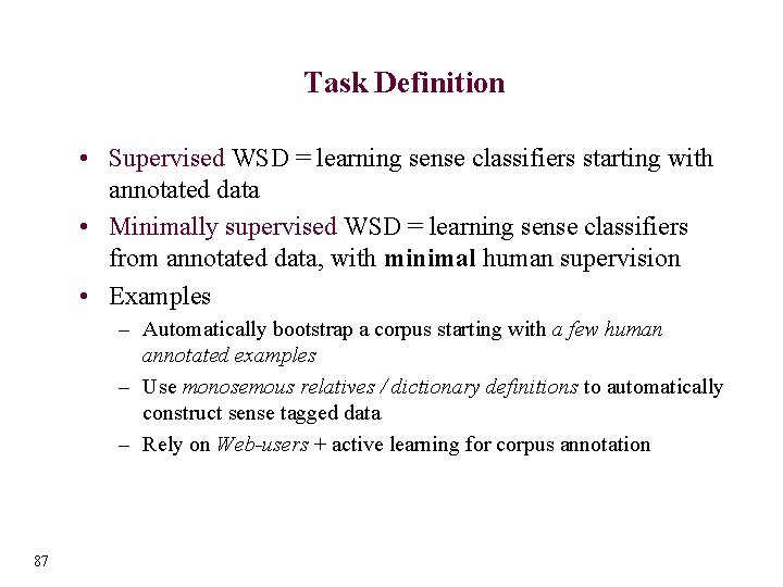
Task Definition • Supervised WSD = learning sense classifiers starting with annotated data • Minimally supervised WSD = learning sense classifiers from annotated data, with minimal human supervision • Examples – Automatically bootstrap a corpus starting with a few human annotated examples – Use monosemous relatives / dictionary definitions to automatically construct sense tagged data – Rely on Web-users + active learning for corpus annotation 87

Outline • Task definition – What does “minimally” supervised mean? • Bootstrapping algorithms – Co-training – Self-training – Yarowsky algorithm • Using the Web for Word Sense Disambiguation – Web as a corpus – Web as collective mind 88

Bootstrapping WSD Classifiers • Build sense classifiers with little training data – Expand applicability of supervised WSD • Bootstrapping approaches – Co-training – Self-training – Yarowsky algorithm 89

Bootstrapping Recipe • Ingredients – (Some) labeled data – (Large amounts of) unlabeled data – (One or more) basic classifiers • Output – Classifier that improves over the basic classifiers 90

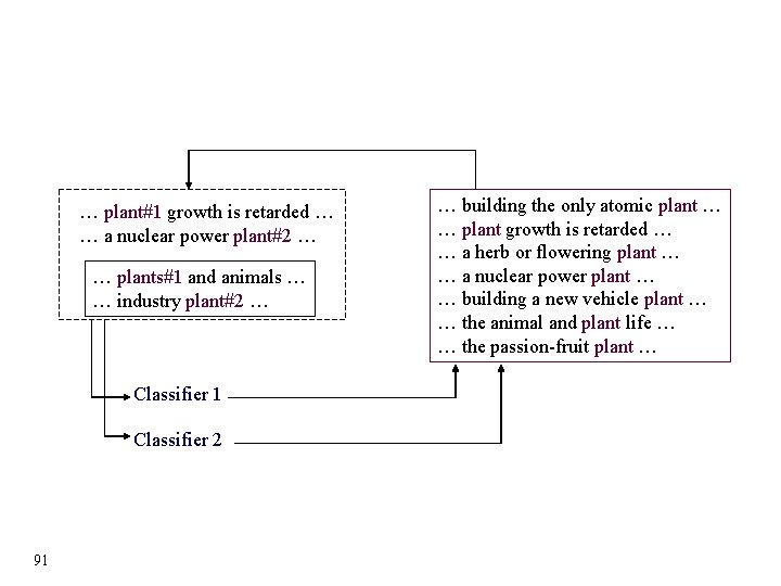
… plant#1 growth is retarded … … a nuclear power plant#2 … … plants#1 and animals … … industry plant#2 … Classifier 1 Classifier 2 91 … building the only atomic plant … … plant growth is retarded … … a herb or flowering plant … … a nuclear power plant … … building a new vehicle plant … … the animal and plant life … … the passion-fruit plant …

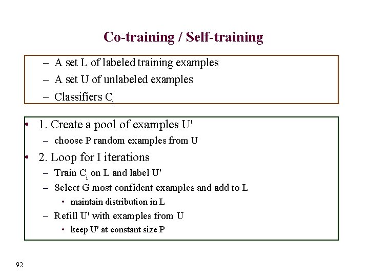
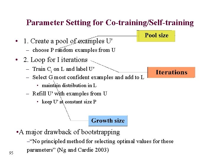
Co-training / Self-training – A set L of labeled training examples – A set U of unlabeled examples – Classifiers Ci • 1. Create a pool of examples U' – choose P random examples from U • 2. Loop for I iterations – Train Ci on L and label U' – Select G most confident examples and add to L • maintain distribution in L – Refill U' with examples from U • keep U' at constant size P 92

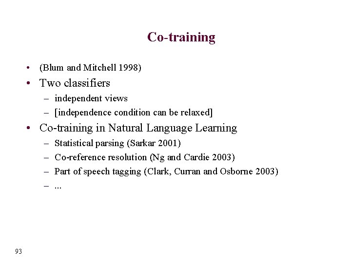
Co-training • (Blum and Mitchell 1998) • Two classifiers – independent views – [independence condition can be relaxed] • Co-training in Natural Language Learning – – 93 Statistical parsing (Sarkar 2001) Co-reference resolution (Ng and Cardie 2003) Part of speech tagging (Clark, Curran and Osborne 2003). . .

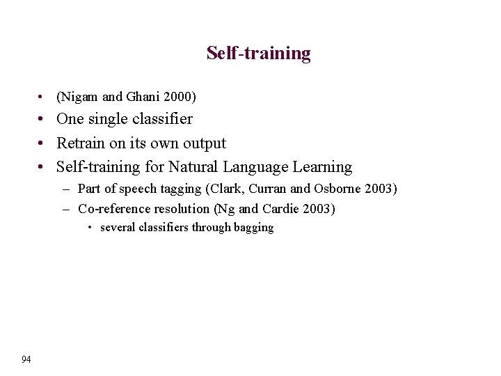
Self-training • (Nigam and Ghani 2000) • One single classifier • Retrain on its own output • Self-training for Natural Language Learning – Part of speech tagging (Clark, Curran and Osborne 2003) – Co-reference resolution (Ng and Cardie 2003) • several classifiers through bagging 94

Parameter Setting for Co-training/Self-training • 1. Create a pool of examples U' – choose P random examples from U • 2. Loop for I iterations – Train Ci on L and label U' – Select G most confident examples and add to L • maintain distribution in L – Refill U' with examples from U • keep U' at constant size P • A major drawback of bootstrapping 95 –“No principled method for selecting optimal values for these parameters” (Ng and Cardie 2003)

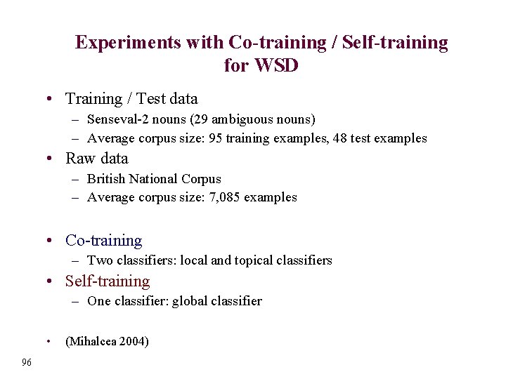
Experiments with Co-training / Self-training for WSD • Training / Test data – Senseval-2 nouns (29 ambiguous nouns) – Average corpus size: 95 training examples, 48 test examples • Raw data – British National Corpus – Average corpus size: 7, 085 examples • Co-training – Two classifiers: local and topical classifiers • Self-training – One classifier: global classifier • 96 (Mihalcea 2004)

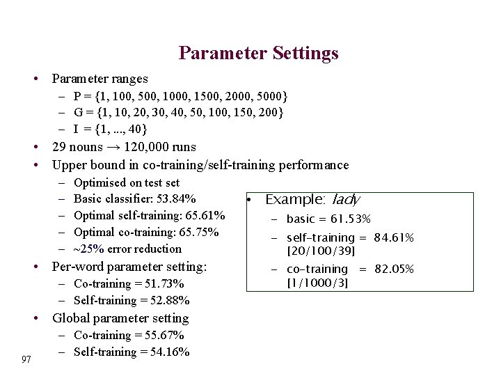
Parameter Settings • Parameter ranges – P = {1, 100, 500, 1000, 1500, 2000, 5000} – G = {1, 10, 20, 30, 40, 50, 100, 150, 200} – I = {1, . . . , 40} • 29 nouns → 120, 000 runs • Upper bound in co-training/self-training performance – – – Optimised on test set Basic classifier: 53. 84% Optimal self-training: 65. 61% Optimal co-training: 65. 75% ~25% error reduction • Per-word parameter setting: – Co-training = 51. 73% – Self-training = 52. 88% • Global parameter setting 97 – Co-training = 55. 67% – Self-training = 54. 16% • Example: lady – basic = 61. 53% – self-training = 84. 61% [20/100/39] – co-training = 82. 05% [1/1000/3]

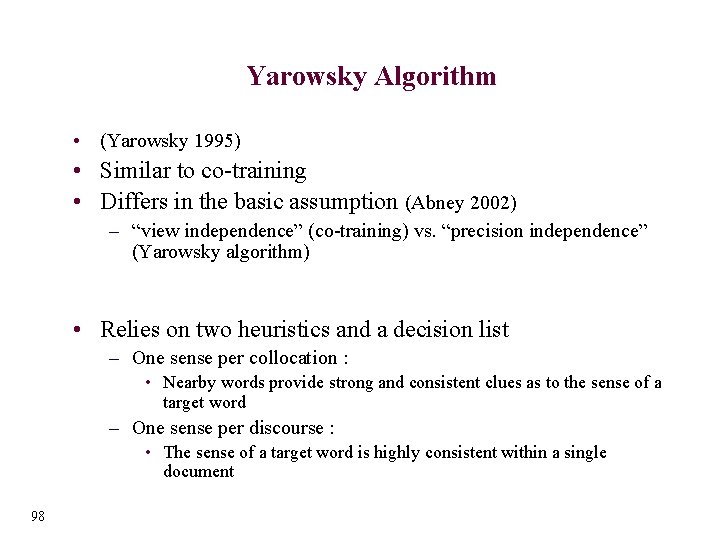
Yarowsky Algorithm • (Yarowsky 1995) • Similar to co-training • Differs in the basic assumption (Abney 2002) – “view independence” (co-training) vs. “precision independence” (Yarowsky algorithm) • Relies on two heuristics and a decision list – One sense per collocation : • Nearby words provide strong and consistent clues as to the sense of a target word – One sense per discourse : • The sense of a target word is highly consistent within a single document 98

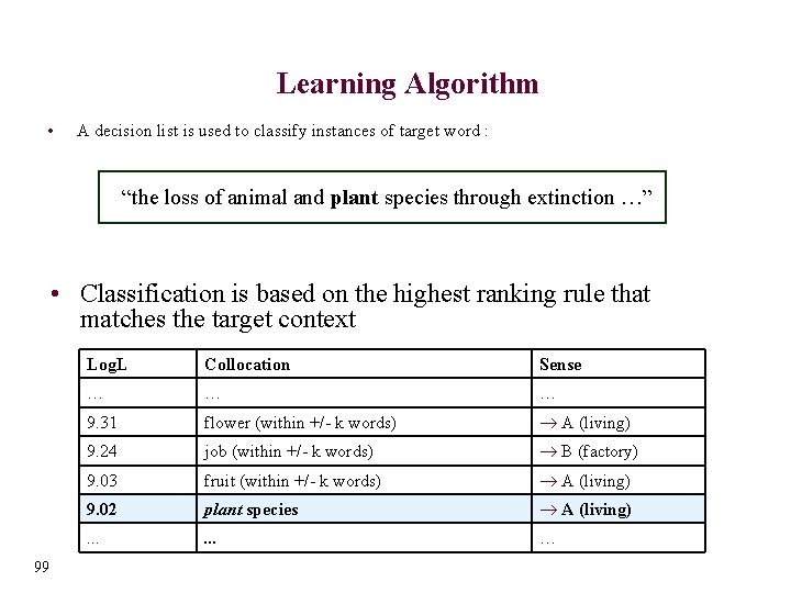
Learning Algorithm • A decision list is used to classify instances of target word : “the loss of animal and plant species through extinction …” • Classification is based on the highest ranking rule that matches the target context 99 Log. L Collocation Sense … … … 9. 31 flower (within +/- k words) ® A (living) 9. 24 job (within +/- k words) ® B (factory) 9. 03 fruit (within +/- k words) ® A (living) 9. 02 plant species ® A (living) . . . …

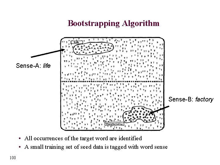
Bootstrapping Algorithm Sense-A: life Sense-B: factory • All occurrences of the target word are identified • A small training set of seed data is tagged with word sense 100

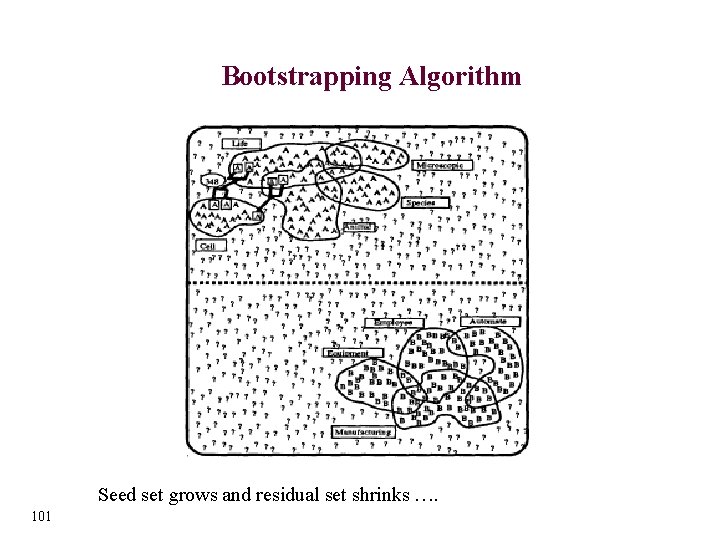
Bootstrapping Algorithm Seed set grows and residual set shrinks …. 101

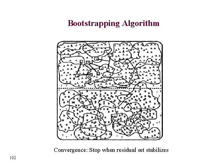
Bootstrapping Algorithm Convergence: Stop when residual set stabilizes 102

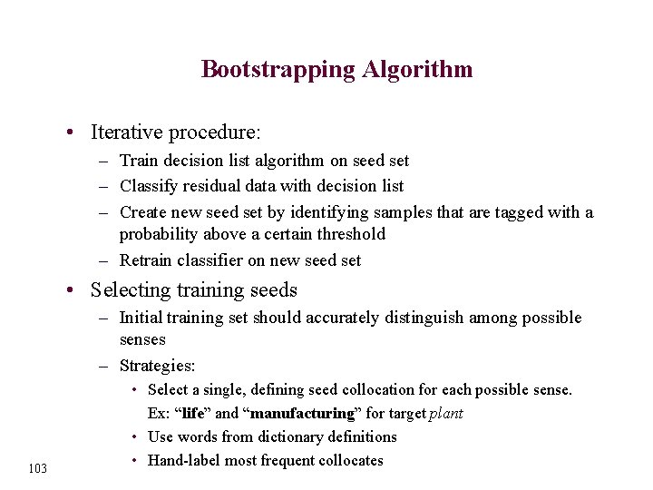
Bootstrapping Algorithm • Iterative procedure: – Train decision list algorithm on seed set – Classify residual data with decision list – Create new seed set by identifying samples that are tagged with a probability above a certain threshold – Retrain classifier on new seed set • Selecting training seeds – Initial training set should accurately distinguish among possible senses – Strategies: 103 • Select a single, defining seed collocation for each possible sense. Ex: “life” and “manufacturing” for target plant • Use words from dictionary definitions • Hand-label most frequent collocates

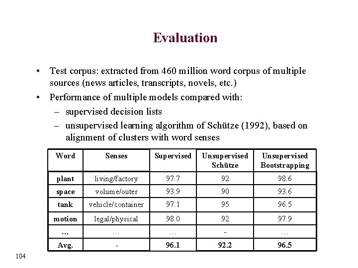
Evaluation • Test corpus: extracted from 460 million word corpus of multiple sources (news articles, transcripts, novels, etc. ) • Performance of multiple models compared with: – supervised decision lists – unsupervised learning algorithm of Schütze (1992), based on alignment of clusters with word senses 104 Word Senses Supervised Unsupervised Schütze Unsupervised Bootstrapping plant living/factory 97. 7 92 98. 6 space volume/outer 93. 9 90 93. 6 tank vehicle/container 97. 1 95 96. 5 motion legal/physical 98. 0 92 97. 9 … … … - … Avg. - 96. 1 92. 2 96. 5

Outline • Task definition – What does “minimally” supervised mean? • Bootstrapping algorithms – Co-training – Self-training – Yarowsky algorithm • Using the Web for Word Sense Disambiguation – Web as a corpus – Web as collective mind 105

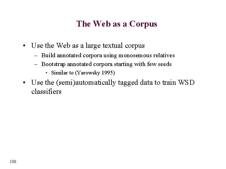
The Web as a Corpus • Use the Web as a large textual corpus – Build annotated corpora using monosemous relatives – Bootstrap annotated corpora starting with few seeds • Similar to (Yarowsky 1995) • Use the (semi)automatically tagged data to train WSD classifiers 106

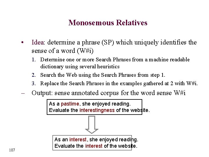
Monosemous Relatives • Idea: determine a phrase (SP) which uniquely identifies the Idea sense of a word (W#i) 1. Determine or more Search Phrases from a machine readable dictionary using several heuristics 2. Search the Web using the Search Phrases from step 1. 3. Replace the Search Phrases in the examples gathered at 2 with W#i. – Output: sense annotated corpus for the word sense W#i As a pastime, she enjoyed reading. Evaluate the interestingness of the website. 107 As an interest, she enjoyed reading. Evaluate the interest of the website.

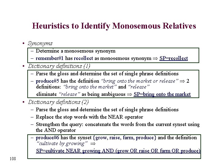
Heuristics to Identify Monosemous Relatives • Synonyms – Determine a monosemous synonym – remember#1 has recollect as monosemous synonym SP=recollect • Dictionary definitions (1) – Parse the gloss and determine the set of single phrase definitions – produce#5 has the definition “bring onto the market or release” 2 definitions: “bring onto the market” and “release” eliminate “release” as being ambiguous SP=bring onto the market • Dictionary defintions (2) – Parse the gloss and determine the set of single phrase definitions – Replace the stop words with the NEAR operator – Strengthen the query: concatenate the words from the current synset using the AND operator – produce#6 has the synset {grow, raise, farm, produce} and the definition “cultivate by growing” SP=cultivate NEAR growing AND (grow OR raise OR farm OR produce) 108

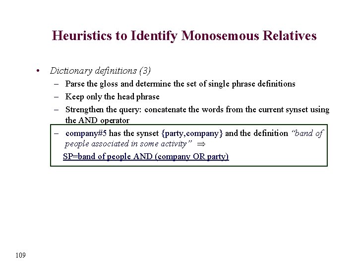
Heuristics to Identify Monosemous Relatives • Dictionary definitions (3) – Parse the gloss and determine the set of single phrase definitions – Keep only the head phrase – Strengthen the query: concatenate the words from the current synset using the AND operator – company#5 has the synset {party, company} and the definition “band of people associated in some activity” SP=band of people AND (company OR party) 109

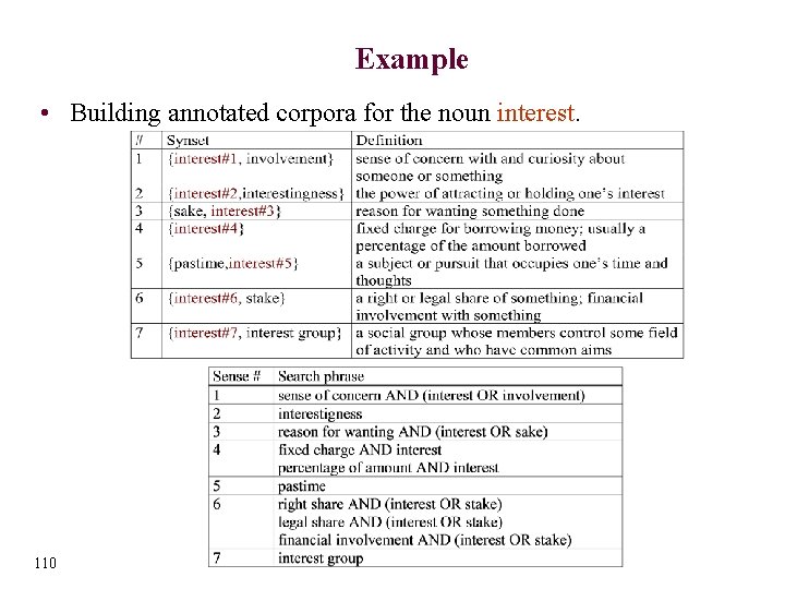
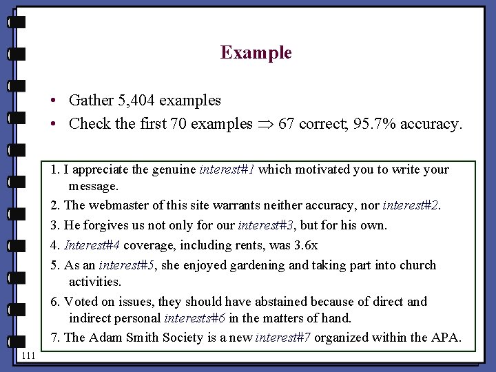
Example • Building annotated corpora for the noun interest. 110

Example • Gather 5, 404 examples • Check the first 70 examples 67 correct; 95. 7% accuracy. 1. I appreciate the genuine interest#1 which motivated you to write your message. 2. The webmaster of this site warrants neither accuracy, nor interest#2. 3. He forgives us not only for our interest#3, but for his own. 4. Interest#4 coverage, including rents, was 3. 6 x 5. As an interest#5, she enjoyed gardening and taking part into church activities. 6. Voted on issues, they should have abstained because of direct and indirect personal interests#6 in the matters of hand. 7. The Adam Smith Society is a new interest#7 organized within the APA. 111

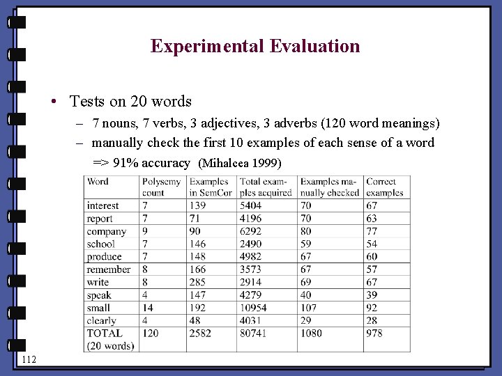
Experimental Evaluation • Tests on 20 words – 7 nouns, 7 verbs, 3 adjectives, 3 adverbs (120 word meanings) – manually check the first 10 examples of each sense of a word => 91% accuracy (Mihalcea 1999) 112

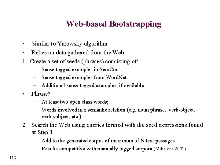
Web-based Bootstrapping • Similar to Yarowsky algorithm • Relies on data gathered from the Web 1. Create a set of seeds (phrases) consisting of: – Sense tagged examples in Sem. Cor – Sense tagged examples from Word. Net – Additional sense tagged examples, if available • Phrase? – At least two open class words; – Words involved in a semantic relation (e. g. noun phrase, verb-object, verb-subject, etc. ) 2. Search the Web using queries formed with the seed expressions found at Step 1 – Add to the generated corpus of maximum of N text passages – Results competitive with manually tagged corpora (Mihalcea 2002) 113

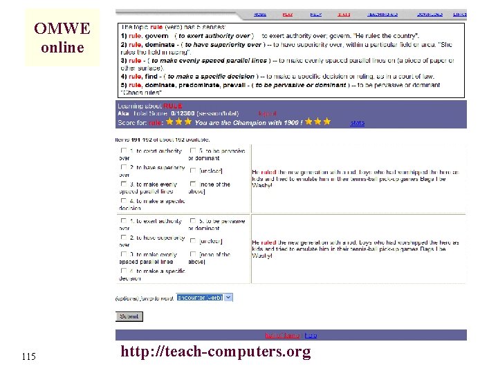
The Web as Collective Mind • Two different views of the Web: – collection of Web pages – very large group of Web users • Millions of Web users can contribute their knowledge to a data repository • Open Mind Word Expert (Chklovski and Mihalcea, 2002) • Fast growing rate: – Started in April 2002 – Currently more than 100, 000 examples of noun senses in several languages 114

OMWE online 115 http: //teach-computers. org

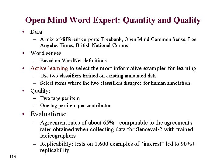
Open Mind Word Expert: Quantity and Quality • Data – A mix of different corpora: Treebank, Open Mind Common Sense, Los Angeles Times, British National Corpus • Word senses – Based on Word. Net definitions • Active learning to select the most informative examples for learning – Use two classifiers trained on existing annotated data – Select items where the two classifiers disagree for human annotation • Quality: – Two tags per item – One tag per item per contributor • Evaluations: – Agreement rates of about 65% - comparable to the agreements rates obtained when collecting data for Senseval-2 with trained lexicographers – Replicability: tests on 1, 600 examples of “interest” led to 90%+ replicability 116

References • • • 117 (Abney 2002) Abney, S. Bootstrapping. Proceedings of ACL 2002. (Blum and Mitchell 1998) Blum, A. and Mitchell, T. Combining labeled and unlabeled data with co-training. Proceedings of COLT 1998. (Chklovski and Mihalcea 2002) Chklovski, T. and Mihalcea, R. Building a sense tagged corpus with Open Mind Word Expert. Proceedings of ACL 2002 workshop on WSD. (Clark, Curran and Osborne 2003) Clark, S. and Curran, J. R. and Osborne, M. Bootstrapping POS taggers using unlabelled data. Proceedings of Co. NLL 2003. (Mihalcea 1999) Mihalcea, R. An automatic method for generating sense tagged corpora. Proceedings of AAAI 1999. (Mihalcea 2002) Mihalcea, R. Bootstrapping large sense tagged corpora. Proceedings of LREC 2002. (Mihalcea 2004) Mihalcea, R. Co-training and Self-training for Word Sense Disambiguation. Proceedings of Co. NLL 2004. (Ng and Cardie 2003) Ng, V. and Cardie, C. Weakly supervised natural language learning without redundant views. Proceedings of HLT-NAACL 2003. (Nigam and Ghani 2000) Nigam, K. and Ghani, R. Analyzing the effectiveness and applicability of co-training. Proceedings of CIKM 2000. (Sarkar 2001) Sarkar, A. Applying cotraining methods to statistical parsing. Proceedings of NAACL 2001. (Yarowsky 1995) Yarowsky, D. Unsupervised word sense disambiguation rivaling supervised methods. Proceedings of ACL 1995.

Part 6: Unsupervised Methods of Word Sense Discrimination

Outline • • • 119 What is Unsupervised Learning? Task Definition Agglomerative Clustering LSI/LSA Sense Discrimination Using Parallel Texts

What is Unsupervised Learning? • Unsupervised learning identifies patterns in a large sample of data, without the benefit of any manually labeled examples or external knowledge sources • These patterns are used to divide the data into clusters, where each member of a cluster has more in common with the other members of its own cluster than any other • Note! If you remove manual labels from supervised data and cluster, you may not discover the same classes as in supervised learning – Supervised Classification identifies features that trigger a sense tag – Unsupervised Clustering finds similarity between contexts 120

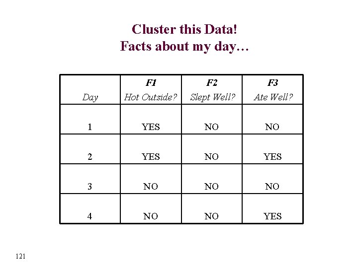
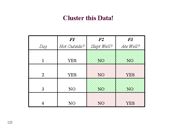
Cluster this Data! Facts about my day… 121 Day F 1 Hot Outside? F 2 Slept Well? F 3 Ate Well? 1 YES NO NO 2 YES NO YES 3 NO NO NO 4 NO NO YES

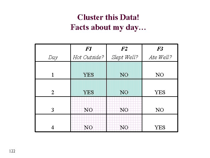
Cluster this Data! Facts about my day… 122 Day F 1 Hot Outside? F 2 Slept Well? F 3 Ate Well? 1 YES NO NO 2 YES NO YES 3 NO NO NO 4 NO NO YES

Cluster this Data! 123 Day F 1 Hot Outside? F 2 Slept Well? F 3 Ate Well? 1 YES NO NO 2 YES NO YES 3 NO NO NO 4 NO NO YES

Outline • • • 124 What is Unsupervised Learning? Task Definition Agglomerative Clustering LSI/LSA Sense Discrimination Using Parallel Texts

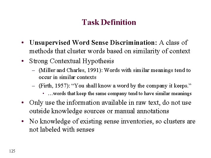
Task Definition • Unsupervised Word Sense Discrimination: A class of methods that cluster words based on similarity of context • Strong Contextual Hypothesis – (Miller and Charles, 1991): Words with similar meanings tend to occur in similar contexts – (Firth, 1957): “You shall know a word by the company it keeps. ” • …words that keep the same company tend to have similar meanings • Only use the information available in raw text, do not use outside knowledge sources or manual annotations • No knowledge of existing sense inventories, so clusters are not labeled with senses 125

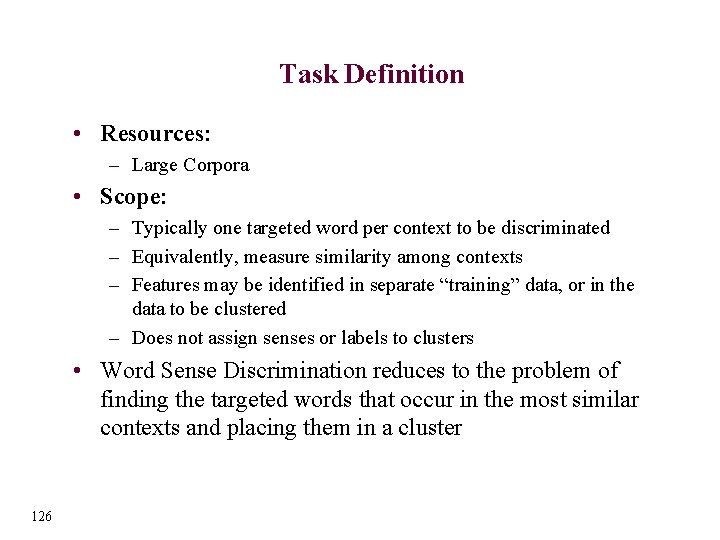
Task Definition • Resources: – Large Corpora • Scope: – Typically one targeted word per context to be discriminated – Equivalently, measure similarity among contexts – Features may be identified in separate “training” data, or in the data to be clustered – Does not assign senses or labels to clusters • Word Sense Discrimination reduces to the problem of finding the targeted words that occur in the most similar contexts and placing them in a cluster 126

Outline • • • 127 What is Unsupervised Learning? Task Definition Agglomerative Clustering LSI/LSA Sense Discrimination Using Parallel Texts

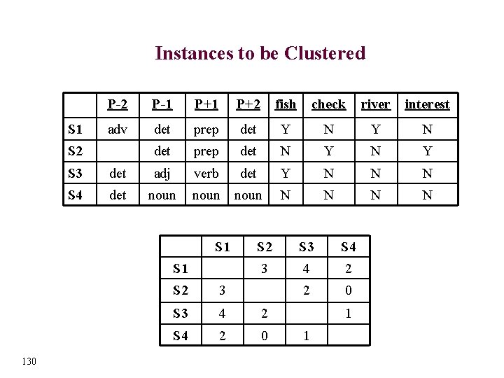
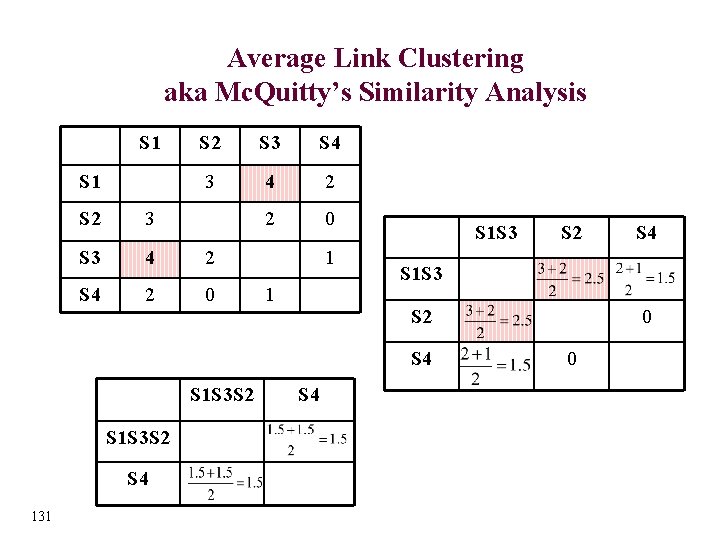
Agglomerative Clustering • Create a similarity matrix of instances to be discriminated – Results in a symmetric “instance by instance” matrix, where each cell contains the similarity score between a pair of instances – Typically a first order representation, where similarity is based on the features observed in the pair of instances • Apply Agglomerative Clustering algorithm to matrix – To start, each instance is its own cluster – Form a cluster from the most similar pair of instances – Repeat until the desired number of clusters is obtained • Advantages : high quality clustering • Disadvantages – computationally expensive, must carry out exhaustive pair wise comparisons 128

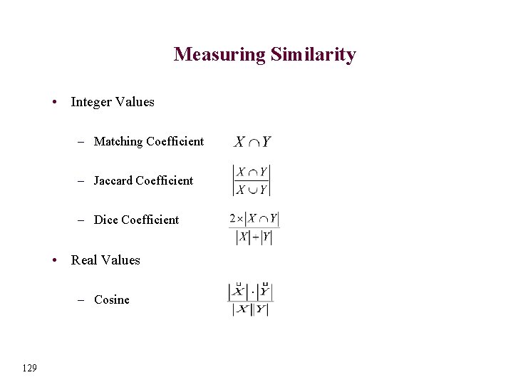
Measuring Similarity • Integer Values – Matching Coefficient – Jaccard Coefficient – Dice Coefficient • Real Values – Cosine 129

Instances to be Clustered S 1 P-2 P-1 P+2 fish check river interest adv det prep det Y N det prep det N Y verb det Y N N N N S 2 S 3 det adj S 4 det noun S 1 130 S 2 S 3 S 4 3 4 2 2 0 S 2 3 S 3 4 2 S 4 2 0 1 1

Average Link Clustering aka Mc. Quitty’s Similarity Analysis S 1 S 2 S 3 S 4 3 4 2 2 0 S 2 3 S 3 4 2 S 4 2 0 1 1 S 1 S 3 S 2 S 4 S 1 S 3 S 2 S 4 131 S 4 0 0

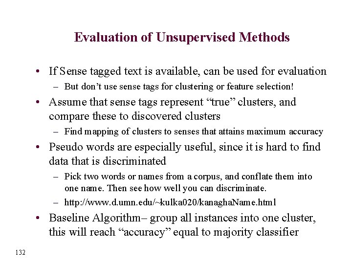
Evaluation of Unsupervised Methods • If Sense tagged text is available, can be used for evaluation – But don’t use sense tags for clustering or feature selection! • Assume that sense tags represent “true” clusters, and compare these to discovered clusters – Find mapping of clusters to senses that attains maximum accuracy • Pseudo words are especially useful, since it is hard to find data that is discriminated – Pick two words or names from a corpus, and conflate them into one name. Then see how well you can discriminate. – http: //www. d. umn. edu/~kulka 020/kanagha. Name. html • Baseline Algorithm– group all instances into one cluster, this will reach “accuracy” equal to majority classifier 132

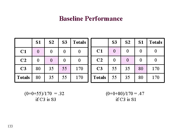
Baseline Performance S 1 S 2 S 3 Totals S 3 S 2 S 1 Totals C 1 0 0 0 0 C 2 0 0 0 0 C 3 80 35 55 170 C 3 55 35 80 170 Totals 80 35 55 170 Totals 55 35 80 170 (0+0+55)/170 =. 32 (0+0+80)/170 =. 47 if C 3 is S 3 if C 3 is S 1 133

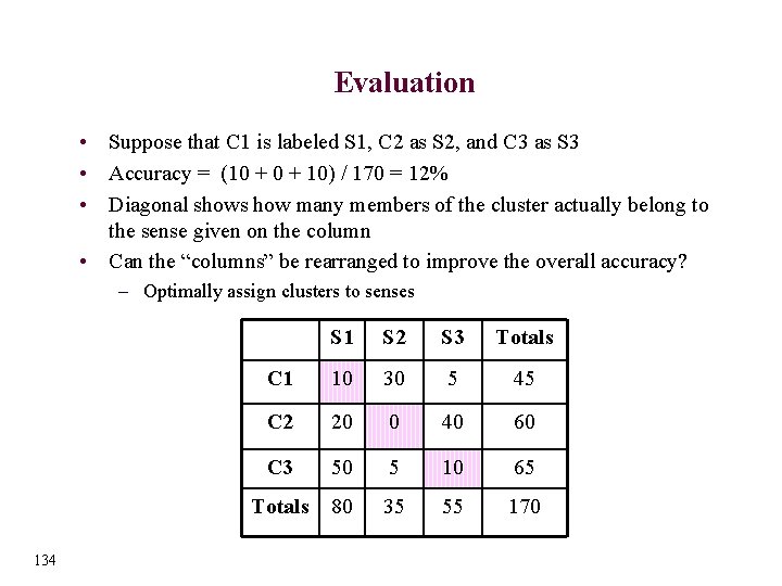
Evaluation • Suppose that C 1 is labeled S 1, C 2 as S 2, and C 3 as S 3 • Accuracy = (10 + 10) / 170 = 12% • Diagonal shows how many members of the cluster actually belong to the sense given on the column • Can the “columns” be rearranged to improve the overall accuracy? – Optimally assign clusters to senses S 1 S 2 S 3 Totals 134 C 1 10 30 5 45 C 2 20 0 40 60 C 3 50 5 10 65 Totals 80 35 55 170

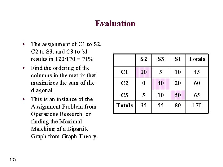
Evaluation • The assignment of C 1 to S 2, C 2 to S 3, and C 3 to S 1 results in 120/170 = 71% • Find the ordering of the columns in the matrix that maximizes the sum of the diagonal. • This is an instance of the Assignment Problem from Operations Research, or finding the Maximal Matching of a Bipartite Graph from Graph Theory. 135 S 2 S 3 S 1 Totals C 1 30 5 10 45 C 2 0 40 20 60 C 3 5 10 50 65 Totals 35 55 80 170

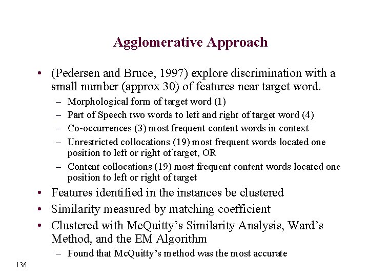
Agglomerative Approach • (Pedersen and Bruce, 1997) explore discrimination with a small number (approx 30) of features near target word. – – Morphological form of target word (1) Part of Speech two words to left and right of target word (4) Co-occurrences (3) most frequent content words in context Unrestricted collocations (19) most frequent words located one position to left or right of target, OR – Content collocations (19) most frequent content words located one position to left or right of target • Features identified in the instances be clustered • Similarity measured by matching coefficient • Clustered with Mc. Quitty’s Similarity Analysis, Ward’s Method, and the EM Algorithm – Found that Mc. Quitty’s method was the most accurate 136

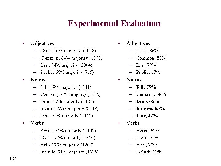
Experimental Evaluation • Adjectives – – • • – – 137 • Agree, 74% majority (1109) Close, 77% majority (1354) Help, 78% majority (1267) Include, 91% majority (1526) • Chief, 86% Common, 80% Last, 79% Public, 63% Nouns – – – Bill, 68% majority (1341) Concern, 64% majority (1235) Drug, 57% majority (1127) Interest, 59% majority (2113) Line, 37% majority (1149) Verbs Adjectives – – Chief, 86% majority (1048) Common, 84% majority (1060) Last, 94% majority (3004) Public, 68% majority (715) Nouns – – – • Bill, 75% Concern, 68% Drug, 65% Interest, 65% Line, 42% Verbs – – Agree, 69% Close, 72% Help, 70% Include, 77%

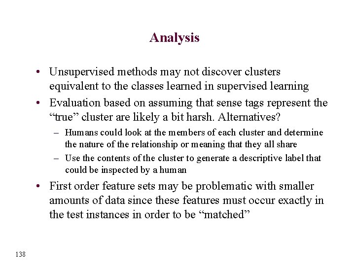
Analysis • Unsupervised methods may not discover clusters equivalent to the classes learned in supervised learning • Evaluation based on assuming that sense tags represent the “true” cluster are likely a bit harsh. Alternatives? – Humans could look at the members of each cluster and determine the nature of the relationship or meaning that they all share – Use the contents of the cluster to generate a descriptive label that could be inspected by a human • First order feature sets may be problematic with smaller amounts of data since these features must occur exactly in the test instances in order to be “matched” 138

Outline • • • 139 What is Unsupervised Learning? Task Definition Agglomerative Clustering LSI/LSA Sense Discrimination Using Parallel Texts

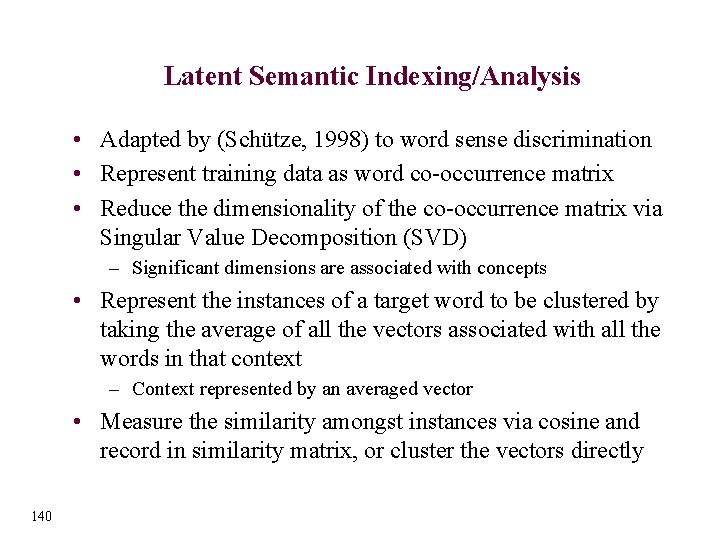
Latent Semantic Indexing/Analysis • Adapted by (Schütze, 1998) to word sense discrimination • Represent training data as word co-occurrence matrix • Reduce the dimensionality of the co-occurrence matrix via Singular Value Decomposition (SVD) – Significant dimensions are associated with concepts • Represent the instances of a target word to be clustered by taking the average of all the vectors associated with all the words in that context – Context represented by an averaged vector • Measure the similarity amongst instances via cosine and record in similarity matrix, or cluster the vectors directly 140

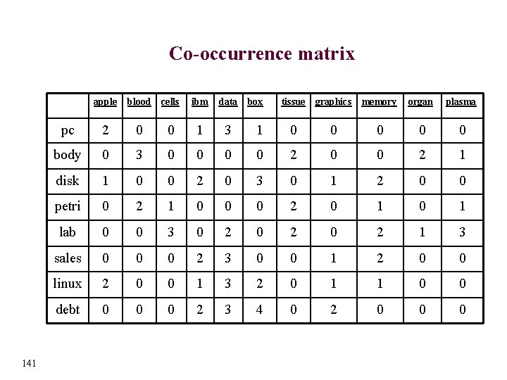
Co-occurrence matrix 141 apple blood cells ibm data pc 2 0 0 1 3 body 0 3 0 0 disk 1 0 0 petri 0 2 lab 0 sales box tissue graphics memory organ plasma 1 0 0 0 0 2 1 2 0 3 0 1 2 0 0 1 0 0 0 2 0 1 0 3 0 2 0 2 1 3 0 0 0 2 3 0 0 1 2 0 0 linux 2 0 0 1 3 2 0 1 1 0 0 debt 0 0 0 2 3 4 0 2 0 0 0

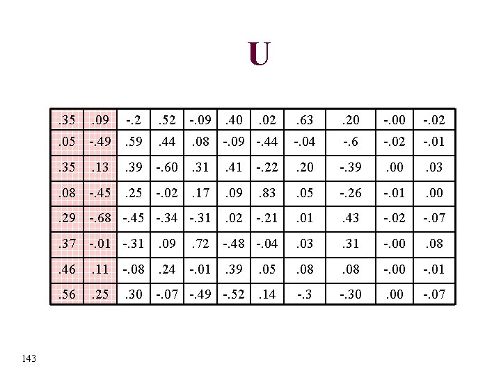
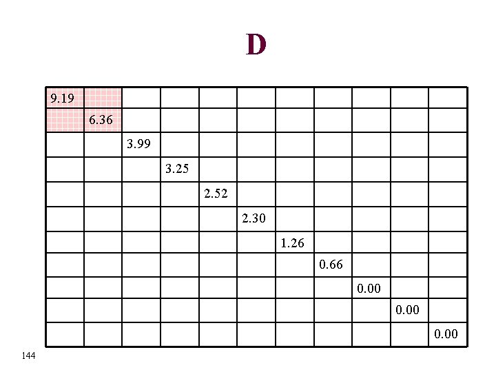
Singular Value Decomposition A=UDV’ 142

U. 35 . 09 -. 2 . 02 . 63 . 20 -. 02 . 08 -. 09 -. 44 -. 04 -. 6 -. 02 -. 01 . 41 -. 22 . 20 -. 39 . 00 . 03 . 09 . 83 . 05 -. 26 -. 01 . 00 . 29 -. 68 -. 45 -. 34 -. 31. 02 -. 21 . 01 . 43 -. 02 -. 07 . 37 -. 01 -. 31. 09 . 03 . 31 -. 00 . 08 . 05 . 08 -. 00 -. 01 . 30 -. 07 -. 49 -. 52. 14 -. 30 . 00 -. 07 . 05 -. 49. 59. 35 . 13 . 52 -. 09. 40. 44 . 39 -. 60. 31 . 08 -. 45. 25 -. 02. 17 143 . 72 -. 48 -. 04 . 46 . 11 -. 08. 24 -. 01. 39 . 56 . 25

D 9. 19 6. 36 3. 99 3. 25 2. 52 2. 30 1. 26 0. 66 0. 00 144

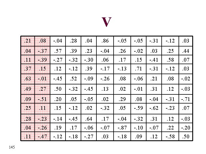
V 145 . 21 . 08 -. 04 . 28 . 04 . 86 -. 05 -. 31 -. 12 . 03 . 04 -. 37 . 57 . 39 . 23 -. 04 . 26 -. 02 . 03 . 25 . 44 . 11 -. 39 -. 27 -. 32 -. 30 . 06 . 17 . 15 -. 41 . 58 . 07 . 37 . 15 . 12 -. 12 . 39 -. 17 -. 13 . 71 -. 31 -. 12 . 03 . 63 -. 01 -. 45 . 52 -. 09 -. 26 . 08 -. 06 . 21 . 08 -. 02 . 49 . 27 . 50 -. 32 -. 45 . 13 . 02 -. 01 . 31 . 12 -. 03 . 09 -. 51 . 20 . 05 -. 05 . 02 . 29 . 08 -. 04 -. 31 -. 71 . 25 . 11 . 15 -. 12 . 02 -. 32 . 05 -. 59 -. 62 -. 23 . 07 . 28 -. 23 -. 14 -. 45 . 64 . 17 -. 04 -. 32 . 31 . 12 -. 03 . 04 -. 26 . 19 . 17 -. 06 -. 07 -. 87 -. 10 -. 07 . 22 -. 20 . 11 -. 47 -. 12 -. 18 -. 27 . 03 -. 18 . 09 . 12 -. 58 . 50

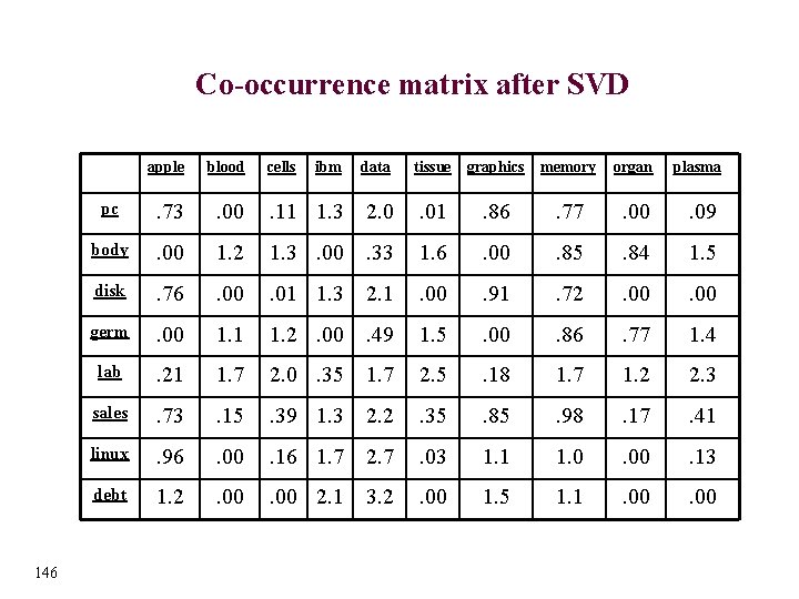
Co-occurrence matrix after SVD 146 apple blood pc . 73 body cells ibm data tissue graphics memory organ plasma . 00 . 11 1. 3 2. 0 . 01 . 86 . 77 . 00 . 09 . 00 1. 2 1. 3. 00. 33 1. 6 . 00 . 85 . 84 1. 5 disk . 76 . 00 . 01 1. 3 2. 1 . 00 . 91 . 72 . 00 germ . 00 1. 1 1. 2. 00. 49 1. 5 . 00 . 86 . 77 1. 4 lab . 21 1. 7 2. 0. 35 1. 7 2. 5 . 18 1. 7 1. 2 2. 3 sales . 73 . 15 . 39 1. 3 2. 2 . 35 . 85 . 98 . 17 . 41 linux . 96 . 00 . 16 1. 7 2. 7 . 03 1. 1 1. 0 . 00 . 13 debt 1. 2 . 00 2. 1 3. 2 . 00 1. 5 1. 1 . 00

Effect of SVD • SVD reduces a matrix to a given number of dimensions This may convert a word level space into a semantic or conceptual space – If “dog” and “collie” and “wolf” are dimensions/columns in the word co-occurrence matrix, after SVD they may be a single dimension that represents “canines” • The dimensions are the principle components that may (hopefully) represent the meaning of concepts • SVD has effect of smoothing a very sparse matrix, so that there are very few 0 valued cells 147

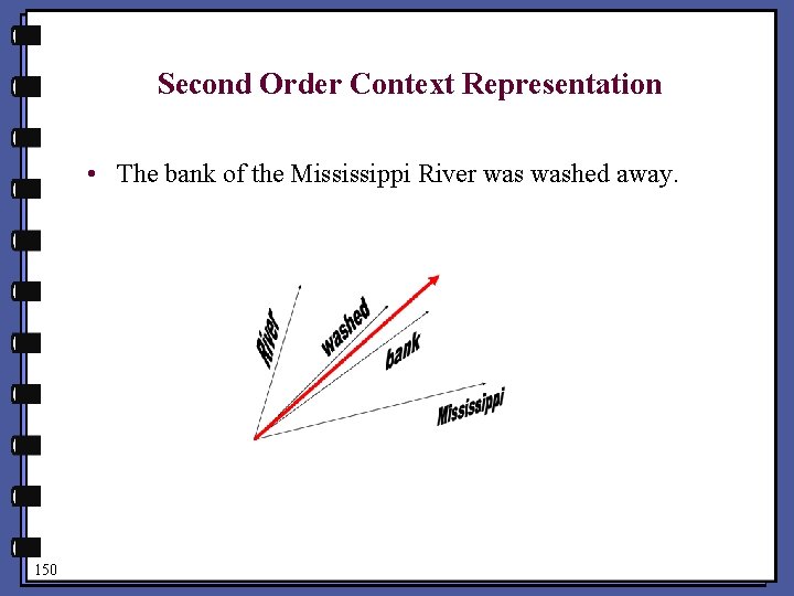
Context Representation • Represent each instance of the target word to be clustered by averaging the word vectors associated with its context – This creates a “second order” representation of the context • The context is represented not only by the words that occur therein, but also the words that occur with the words in the context elsewhere in the training corpus 148

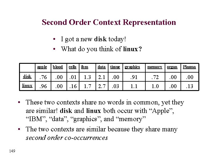
Second Order Context Representation • I got a new disk today! • What do you think of linux? apple blood cells disk . 76 . 00 . 01 linux . 96 . 00 . 16 ibm data tissue 1. 3 2. 1 . 00 1. 7 2. 7 . 03 graphics memory organ Plasma . 91 . 72 . 00 1. 1 1. 0 . 00 . 13 • These two contexts share no words in common, yet they are similar! disk and linux both occur with “Apple”, “IBM”, “data”, “graphics”, and “memory” • The two contexts are similar because they share many second order co-occurrences 149

Second Order Context Representation • The bank of the Mississippi River washed away. 150

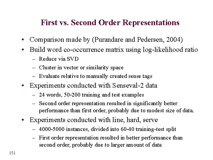
First vs. Second Order Representations • Comparison made by (Purandare and Pedersen, 2004) • Build word co-occurrence matrix using log-likelihood ratio – Reduce via SVD – Cluster in vector or similarity space – Evaluate relative to manually created sense tags • Experiments conducted with Senseval-2 data – 24 words, 50 -200 training and test examples – Second order representation resulted in significantly better performance than first order, probably due to modest size of data. • Experiments conducted with line, hard, serve – 4000 -5000 instances, divided into 60 -40 training-test split – First order representation resulted in better performance than second order, probably due to larger amount of data 151

Analysis • Agglomerative methods based on direct (first order) features require large amounts of data in order to obtain a reliable set of features • Large amounts of data are problematic for agglomerative clustering (due to exhaustive comparisons) • Second order representations allow you to make due with smaller amounts of data, and still get a rich (non-sparse) representation of context • http: //senseclusters. sourceforge. net is a complete system for performing unsupervised discrimination using first or second order context vectors in similarity or vector space, and includes support for SVD, clustering and evaluation 152

Outline • • • 153 What is Unsupervised Learning? Task Definition Agglomerative Clustering LSI/LSA Sense Discrimination Using Parallel Texts

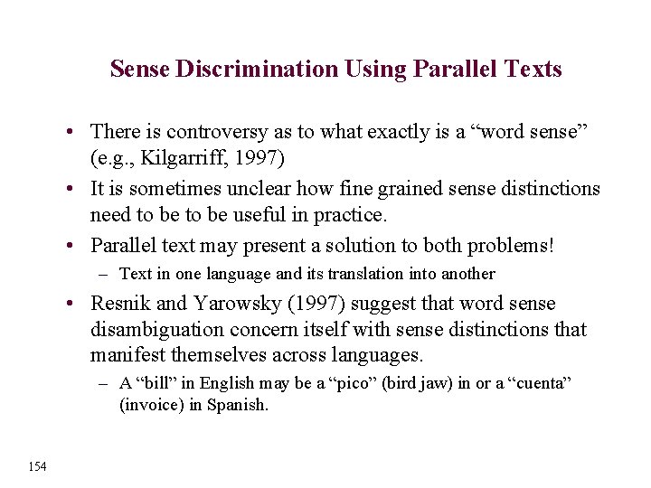
Sense Discrimination Using Parallel Texts • There is controversy as to what exactly is a “word sense” (e. g. , Kilgarriff, 1997) • It is sometimes unclear how fine grained sense distinctions need to be useful in practice. • Parallel text may present a solution to both problems! – Text in one language and its translation into another • Resnik and Yarowsky (1997) suggest that word sense disambiguation concern itself with sense distinctions that manifest themselves across languages. – A “bill” in English may be a “pico” (bird jaw) in or a “cuenta” (invoice) in Spanish. 154

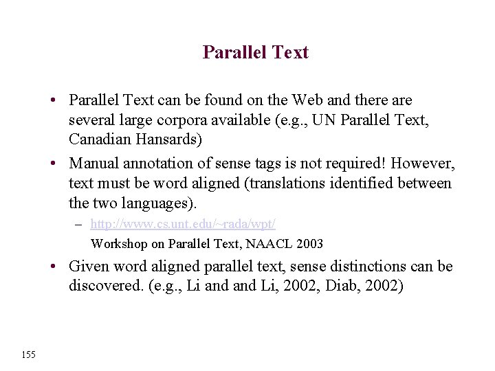
Parallel Text • Parallel Text can be found on the Web and there are several large corpora available (e. g. , UN Parallel Text, Canadian Hansards) • Manual annotation of sense tags is not required! However, text must be word aligned (translations identified between the two languages). – http: //www. cs. unt. edu/~rada/wpt/ Workshop on Parallel Text, NAACL 2003 • Given word aligned parallel text, sense distinctions can be discovered. (e. g. , Li and Li, 2002, Diab, 2002) 155

References • • • 156 (Diab, 2002) Diab, Mona and Philip Resnik, An Unsupervised Method for Word Sense Tagging using Parallel Corpora, Proceedings of ACL, 2002. (Firth, 1957) A Synopsis of Linguistic Theory 1930 -1955. In Studies in Linguistic Analysis, Oxford University Press, Oxford. (Kilgarriff, 1997) “I don’t believe in word senses”, Computers and the Humanities (31) pp. 91 -113. (Li and Li, 2002) Word Translation Disambiguation Using Bilingual Bootstrapping. Proceedings of ACL. Pp. 343 -351. (Mc. Quitty, 1966) Similarity Analysis by Reciprocal Pairs for Discrete and Continuous Data. Educational and Psychological Measurement (26) pp. 825 -831. (Miller and Charles, 1991) Contextual correlates of semantic similarity. Language and Cognitive Processes, 6 (1) pp. 1 - 28. (Pedersen and Bruce, 1997) Distinguishing Word Sense in Untagged Text. In Proceedings of EMNLP 2. pp 197 -207. (Purandare and Pedersen, 2004) Word Sense Discrimination by Clustering Contexts in Vector and Similarity Spaces. Proceedings of the Conference on Natural Language and Learning. pp. 41 -48. (Resnik and Yarowsky, 1997) A Perspective on Word Sense Disambiguation Methods and their Evaluation. The ACL-SIGLEX Workshop Tagging Text with Lexical Semantics. pp. 79 -86. (Schutze, 1998) Automatic Word Sense Discrimination. Computational Linguistics, 24 (1) pp. 97 -123.

Part 7: How to Get Started in Word Sense Disambiguation Research

Outline • Where to get the required ingredients? – – Machine Readable Dictionaries Machine Learning Algorithms Sense Annotated Data Raw Data • Where to get WSD software? • How to get your algorithms tested? – Senseval 158

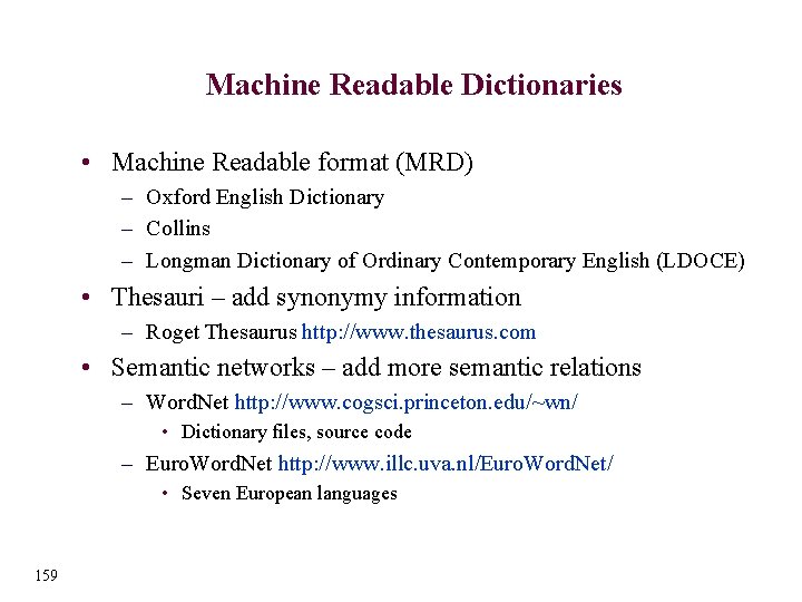
Machine Readable Dictionaries • Machine Readable format (MRD) – Oxford English Dictionary – Collins – Longman Dictionary of Ordinary Contemporary English (LDOCE) • Thesauri – add synonymy information – Roget Thesaurus http: //www. thesaurus. com • Semantic networks – add more semantic relations – Word. Net http: //www. cogsci. princeton. edu/~wn/ • Dictionary files, source code – Euro. Word. Net http: //www. illc. uva. nl/Euro. Word. Net/ • Seven European languages 159

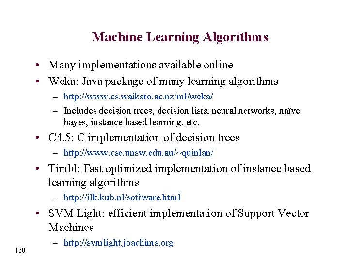
Machine Learning Algorithms • Many implementations available online • Weka: Java package of many learning algorithms – http: //www. cs. waikato. ac. nz/ml/weka/ – Includes decision trees, decision lists, neural networks, naïve bayes, instance based learning, etc. • C 4. 5: C implementation of decision trees – http: //www. cse. unsw. edu. au/~quinlan/ • Timbl: Fast optimized implementation of instance based learning algorithms – http: //ilk. kub. nl/software. html • SVM Light: efficient implementation of Support Vector Machines 160 – http: //svmlight. joachims. org

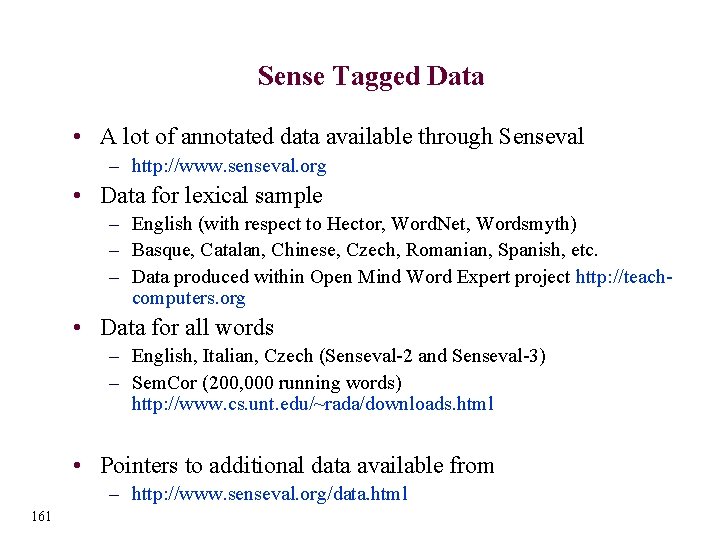
Sense Tagged Data • A lot of annotated data available through Senseval – http: //www. senseval. org • Data for lexical sample – English (with respect to Hector, Word. Net, Wordsmyth) – Basque, Catalan, Chinese, Czech, Romanian, Spanish, etc. – Data produced within Open Mind Word Expert project http: //teachcomputers. org • Data for all words – English, Italian, Czech (Senseval-2 and Senseval-3) – Sem. Cor (200, 000 running words) http: //www. cs. unt. edu/~rada/downloads. html • Pointers to additional data available from – http: //www. senseval. org/data. html 161

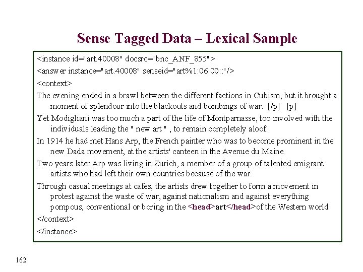
Sense Tagged Data – Lexical Sample <instance id="art. 40008" docsrc="bnc_ANF_855"> <answer instance="art. 40008" senseid="art%1: 06: 00: : "/> <context> The evening ended in a brawl between the different factions in Cubism, but it brought a moment of splendour into the blackouts and bombings of war. [/p] [p] Yet Modigliani was too much a part of the life of Montparnasse, too involved with the individuals leading the " new art " , to remain completely aloof. In 1914 he had met Hans Arp, the French painter who was to become prominent in the new Dada movement, at the artists' canteen in the Avenue du Maine. Two years later Arp was living in Zurich, a member of a group of talented emigrant artists who had left their own countries because of the war. Through casual meetings at cafes, the artists drew together to form a movement in protest against the waste of war, against nationalism and against everything pompous, conventional or boring in the <head>art</head>of the Western world. </context> </instance> 162

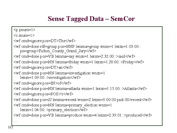
Sense Tagged Data – Sem. Cor <p pnum=1> <s snum=1> <wf cmd=ignore pos=DT>The</wf> <wf cmd=done rdf=group pos=NNP lemma=group wnsn=1 lexsn=1: 03: 00: : pn=group>Fulton_County_Grand_Jury</wf> <wf cmd=done pos=VB lemma=say wnsn=1 lexsn=2: 32: 00: : >said</wf> <wf cmd=done pos=NN lemma=friday wnsn=1 lexsn=1: 28: 00: : >Friday</wf> <wf cmd=ignore pos=DT>an</wf> <wf cmd=done pos=NN lemma=investigation wnsn=1 lexsn=1: 09: 00: : >investigation</wf> <wf cmd=ignore pos=IN>of</wf> <wf cmd=done pos=NN lemma=atlanta wnsn=1 lexsn=1: 15: 00: : >Atlanta</wf> <wf cmd=ignore pos=POS>'s</wf> <wf cmd=done pos=JJ lemma=recent wnsn=2 lexsn=5: 00: past: 00>recent</wf> <wf cmd=done pos=NN lemma=primary_election wnsn=1 lexsn=1: 04: 00: : >primary_election</wf> <wf cmd=done pos=VB lemma=produce wnsn=4 lexsn=2: 39: 01: : >produced</wf> … 163

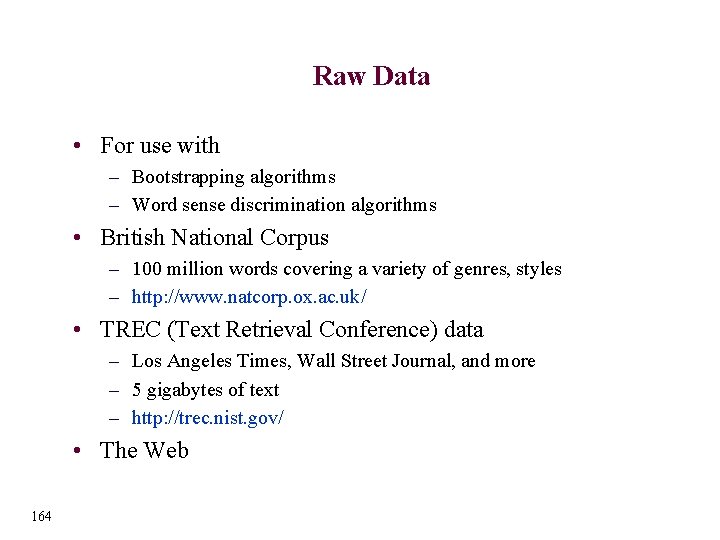
Raw Data • For use with – Bootstrapping algorithms – Word sense discrimination algorithms • British National Corpus – 100 million words covering a variety of genres, styles – http: //www. natcorp. ox. ac. uk/ • TREC (Text Retrieval Conference) data – Los Angeles Times, Wall Street Journal, and more – 5 gigabytes of text – http: //trec. nist. gov/ • The Web 164

Outline • Where to get the required ingredients? – – Machine Readable Dictionaries Machine Learning Algorithms Sense Annotated Data Raw Data • Where to get WSD software? • How to get your algorithms tested? – Senseval 165

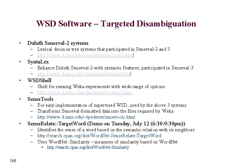
WSD Software – Targeted Disambiguation • Duluth Senseval-2 systems – Lexical decision tree systems that participated in Senseval-2 and 3 – http: //www. d. umn. edu/~tpederse/senseval 2. html • Synta. Lex – Enhance Duluth Senseval-2 with syntactic features, participated in Senseval-3 – http: //www. d. umn. edu/~tpederse/syntalex. html • WSDShell – Shell for running Weka experiments with wide range of options – http: //www. d. umn. edu/~tpederse/wsdshell. html • Sense. Tools – For easy implementation of supervised WSD, used by the above 3 systems – Transforms Senseval-formatted data into the files required by Weka – http: //www. d. umn. edu/~tpederse/sensetools. html • Sense. Relate: : Target. Word (Demo on Tuesday, July 12 (6: 30 -9: 30 pm)) – Identifies the sense of a word based on the semantic relation with its neighbors – http: //search. cpan. org/dist/Word. Net-Sense. Relate-Target. Word – Uses Word. Net: : Similarity – measures of similarity based on Word. Net • http: //search. cpan. org/dist/Word. Net-Similarity 166

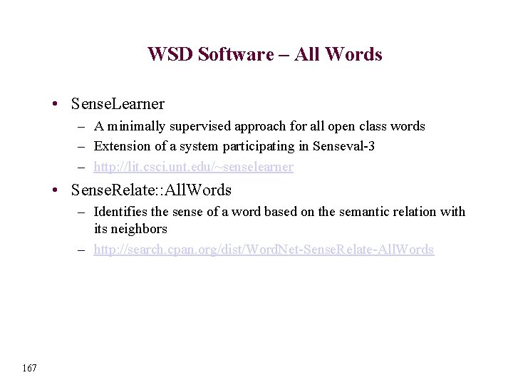
WSD Software – All Words • Sense. Learner – A minimally supervised approach for all open class words – Extension of a system participating in Senseval-3 – http: //lit. csci. unt. edu/~senselearner • Sense. Relate: : All. Words – Identifies the sense of a word based on the semantic relation with its neighbors – http: //search. cpan. org/dist/Word. Net-Sense. Relate-All. Words 167

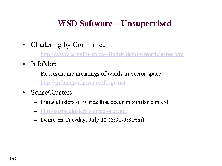
WSD Software – Unsupervised • Clustering by Committee – http: //www. cs. ualberta. ca/~lindek/demos/wordcluster. htm • Info. Map – Represent the meanings of words in vector space – http: //infomap-nlp. sourceforge. net • Sense. Clusters – Finds clusters of words that occur in similar context – http: //senseclusters. sourceforge. net – Demo on Tuesday, July 12 (6: 30 -9: 30 pm) 168

Outline • Where to get the required ingredients? – – Machine Readable Dictionaries Machine Learning Algorithms Sense Annotated Data Raw Data • Where to get WSD software? • How to get your algorithms tested? – Senseval 169

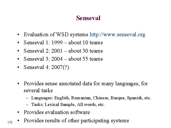
Senseval • • • Evaluation of WSD systems http: //www. senseval. org Senseval 1: 1999 – about 10 teams Senseval 2: 2001 – about 30 teams Senseval 3: 2004 – about 55 teams Senseval 4: 2007(? ) • Provides sense annotated data for many languages, for several tasks – Languages: English, Romanian, Chinese, Basque, Spanish, etc. – Tasks: Lexical Sample, All words, etc. 170 • Provides evaluation software • Provides results of other participating systems

Senseval 171

Part 8: Conclusions

Outline • • 173 The Web and WSD Multilingual WSD The Next Five Years (2005 -2010) Concluding Remarks

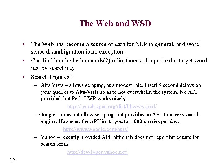
The Web and WSD • The Web has become a source of data for NLP in general, and word sense disambiguation is no exception. • Can find hundreds/thousands(? ) of instances of a particular target word just by searching. • Search Engines : – Alta Vista – allows scraping, at a modest rate. Insert 5 second delays on your queries to Alta-Vista so as to not overwhelm the system. No API provided, but Perl: : LWP works nicely. http: //search. cpan. org/dist/libwww-perl/ -- Google – does not allow scraping, but provides an API to access search engine. However, the API limits you to 1, 000 queries per day. http: //www. google. com/apis/ – Yahoo – recently provided API, although does not report hit counts for search terms http: //developer. yahoo. net/ 174

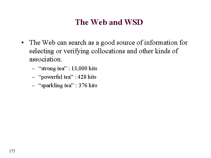
The Web and WSD • The Web can search as a good source of information for selecting or verifying collocations and other kinds of association. – “strong tea” : 13, 000 hits – “powerful tea” : 428 hits – “sparkling tea” : 376 hits 175

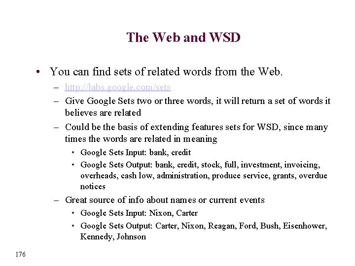
The Web and WSD • You can find sets of related words from the Web. – http: //labs. google. com/sets – Give Google Sets two or three words, it will return a set of words it believes are related – Could be the basis of extending features sets for WSD, since many times the words are related in meaning • Google Sets Input: bank, credit • Google Sets Output: bank, credit, stock, full, investment, invoicing, overheads, cash low, administration, produce service, grants, overdue notices – Great source of info about names or current events • Google Sets Input: Nixon, Carter • Google Sets Output: Carter, Nixon, Reagan, Ford, Bush, Eisenhower, Kennedy, Johnson 176

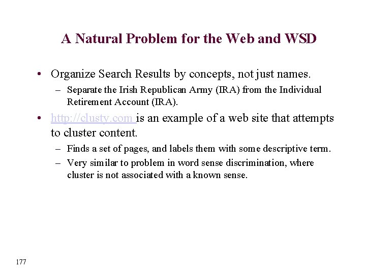
A Natural Problem for the Web and WSD • Organize Search Results by concepts, not just names. – Separate the Irish Republican Army (IRA) from the Individual Retirement Account (IRA). • http: //clusty. com is an example of a web site that attempts to cluster content. – Finds a set of pages, and labels them with some descriptive term. – Very similar to problem in word sense discrimination, where cluster is not associated with a known sense. 177

The Web and WSD, not all good news • Lots and lots of junk to filter through. Lots of misleading and malicious content on web pages. • Counts as reported by search engines for hits are approximations and vary sometime from query to query. Over time they will change, so it’s very hard to reproduce experimental results over time. • Search engines could close down API, prohibit scraping, etc. – there are no promises made. • Can be slow to get data from the Web. 178

Outline • • 179 The Web and WSD Multilingual WSD The Next Five Years (2005 -2010) Concluding Remarks

Multilingual WSD • Parallel text is a potential meeting ground between raw untagged text (like unsupervised methods use) and sense tagged text (like the supervised methods need) • A source language word that is translated into various different target language forms may be polysemous in the source language 180

A Clever Way to Sense Tag • Expertise of native speakers can be used to create sense tagged text, without having to refer to dictionaries! • Have a bilingual native speaker pick the proper translation for a word in a given context. http: //www. teach-computers. org/word-expert/english-hindi/ http: //www. teach-computers. org/word-expert/english-french/ • This is a much more intuitive way to sense tag text, and depends only on the native speakers expertise, not a set of senses as found in a particular dictionary. 181

Outline • • 182 The Web and WSD Multilingual WSD The Next Five Years (2005 -2010) Concluding Remarks

The Next Five Years • Applications, applications, and applications. Where are the applications? WSD needs to demonstrate an impact on applications in the next five years. • Word Sense Disambiguation will be deployed in an increasing number of applications over the next five years. – However, not in Machine Translation. Too difficult to integrate WSD into current statistical systems, and this won’t change soon. – Most likely applications include web search tools and email organizers and search tools (like gmail). • If you are writing papers, “bake off” evaluations will meet with more rejection that acceptance • If you have a potential application for Word Sense Disambiguation in any of its forms, tell us!! Please! 183

Outline • • 184 The Web and WSD Multilingual WSD The Next Five Years (2005 -2010) Concluding Remarks

Concluding Remarks • Word Sense Disambiguation has something for everyone! – – – – Statistical Methods Knowledge Based systems Supervised Machine Learning Unsupervised Learning Semi-Supervised Bootstrapping and Co-training Human Annotation of Data • The impact of high quality WSD will be huge. NLP consumers have become accustomed to systems that only make coarse grained distinctions between concepts, or who might not make any at all. • Real Understanding? Real AI? 185

Thank You! • Rada Mihalcea (rada@cs. unt. edu) – http: //www. cs. unt. edu/~rada • Ted Pedersen (tpederse@d. umn. edu) – http: //www. d. umn. edu/~tpederse 186