VIII Factorial designs at two levels VIII A

Factorial designs at two levels • • Definition VIII. 1: An experiment that involves

VIII. A Replicated 2 k experiments • An experiment involving three factors — a

Notations for treatment combinations • Definition VIII. 2: There are three systems of specifying

Example VIII. 1 23 pilot plant experiment • An experimenter conducted a 23 experiment

Getting data into R • As before, use fac. layout. First consideration is: –

Result of expressions > Fac 3 Pilot. dat <data. frame(Fac 3 Pilot. lay, Yield

b) Analysis of variance • The analysis of replicated 2 k factorial experiments is

Example VIII. 1 23 pilot plant experiment (continued) The features of this experiment are

• Sources derived from randomized structure formula: Temp*Conc*Catal = Temp + (Conc*Catal) +

R output: > attach(Fac 3 Pilot. dat) > interaction. ABC. plot(Yield, Te, C, K,

R (continued) > Fac 3 Pilot. aov <- aov(Yield ~ Te * C *

R output (continued) > > > # # Diagnostic checking # res <- resid.

R output (continued) • These plots are fine Statistical Modelling Chapter VIII 14

R output (continued) • All the residuals plots appear to be satisfactory. Statistical Modelling

The hypothesis test for this experiment Step 1: Set up hypotheses a) H 0:

Hypothesis test (continued) Step 2: Calculate test statistics • ANOVA table for 3 -factorial

Conclusions • Yield depends on particular combination of Temp and Catalyst, whereas Concentration also

c) Calculation of responses and Yates effects • When all the factors in a

Calculation of effects (continued) • Two-factor interactions, elements of (a b)e, (a c)e and

Simplifying the B#C interaction effect for i = 1, j = 1 Statistical Modelling

All 4 effects • Again only one independent quantity and so 1 df. •

Calculation of effects (continued) • All effects in a 2 k experiment have only

Responses and Yates effects • Definition VIII. 3: A one-factor response and a Yates

Computation of sums of squares • Definition VIII. 6: Sums of squares can be

Example VIII. 1 23 pilot plant experiment (continued) • Obtain responses and Yates interaction

Example VIII. 1 23 pilot plant experiment (continued) • Two-factor T#K response is –

Example VIII. 1 23 pilot plant experiment (continued) • T#K interaction effect can be

Summary Statistical Modelling Chapter VIII 29

Example: T#C#K interaction • Can show that the three-factor Yates interaction effect consists of

Easy rules for determining the signs of observations to compute the Yates effects •

Example VIII. 1 23 pilot plant experiment (continued) • Useful in calculating responses, effects

Using R to get Yates effects • A table of Yates effects can be

d) Yates algorithm • See notes Statistical Modelling Chapter VIII 34

e) Treatment differences Mean differences • Examine tables of means corresponding to the terms

Tables of means • For T K combinations. • Temperature difference less without the

Which treatments would give the highest yield? • Highest yielding combination of temperature and

Which treatments would give the highest yield? • So combination of factors that will

Polynomial models and fitted values • As only 2 levels of each factor, a

Fitted values for X with ± 1 Definition VIII. 8: The fitted values are

Example VIII. 1 23 pilot plant experiment (continued) • For the example, the significant

Example VIII. 1 23 pilot plant experiment (continued) • We can write an element

Optimum yield • The optimum yield occurs for T and K high and C

VIII. B Economy in experimentation • Run 2 k experiments unreplicated. • Apparent problem:

a) Design of unreplicated 2 k experiments, including R expressions • As there is

Generating the layout for an unreplicated 23 experiment > > > + + +

Example VIII. 2 A 24 process development study • The data given in the

b) Initial analysis of variance • All possible interactions Example VIII. 2 A 24

Example VIII. 2 A 24 process development study (continued) > Fac 4 Proc. aov

c) Analysis assuming no 3 -factor or 4 -factor interactions • However, if we

Example VIII. 2 A 24 process development study (continued) R output > # Perform

Example VIII. 2 A 24 process development study (continued) • The analysis is summarized

Example VIII. 2 A 24 process development study (continued) • However, there is a

d) Probability plot of Yates effects • A method that: – does not require

Example VIII. 2 A 24 process development study (continued) > #Yates effects probability plot

Example VIII. 2 A 24 process development study (continued) • The large Yates effects

e) Fitted values Example VIII. 2 A 24 process development study (continued) • Grand

Example VIII. 2 A 24 process development study (continued) • For example, the predicted

f) Diagnostic checking • Having determined the significant terms, one can – reanalyze with

Example VIII. 2 A 24 process development study (continued) > > # # Diagnostic

Example VIII. 2 A 24 process development study (continued) • The residual-versus-fitted-values and residuals-versus-factors

Example VIII. 2 A 24 process development study (continued) Statistical Modelling Chapter VIII 62

g) Treatment differences • As a result of the analysis we have – identified

Example VIII. 2 A 24 process development study (continued) The R output that examines

Examine Temp-Conc means > interaction. plot(Temp, Conc, Conv) > q <- qtukey(0. 95, 4,

Conclusion • From the tables of means it is concluded that the maximum conversion

VIII. C Confounding in factorial experiments a) Total confounding of effects • Not always

Example VIII. 3 Complete sets of factorial treatments in 2 blocks • Suppose that

Example VIII. 3 Complete sets of factorial treatments in 2 blocks (continued) • Divide

The experimental structure and analysis of variance table • In this experiment, we have

Example VIII. 4 Repeated two block experiment • To increase precision could replicate the

Example VIII. 4 Repeated two block experiment (continued) • The experimental structure for the

Example VIII. 5 Complete sets of factorial treatments in 4 blocks • Suppose that

Example VIII. 5 Complete sets of factorial treatments in 4 blocks (continued) • The

Example VIII. 5 Complete sets of factorial treatments in 4 blocks (continued) • There

Calculus for finding confounding • Theorem VIII. 1: Let the columns in a table

Example VIII. 5 Complete sets of factorial treatments in 4 blocks (continued) • Firstly,

Example VIII. 5 Complete sets of factorial treatments in 4 blocks (continued) • A

Blocks made up of fold-over pairs. • Definition VIII. 11: Two factor combinations are

Example VIII. 6: Repeated four block experiment • As before could replicate so that

Example VIII. 6: Repeated four block experiment (continued) • Analysis indicates that the two-factor

b) Partial confounding of effects • In experiments where the complete set of treatments

Example VIII. 7 Partial confounding in a repeated four block experiment • Suppose that

Formation of the groups of treatments Statistical Modelling Chapter VIII 86

Randomization • Randomize – groups (pairs) of treatments to the blends – 2 treatment

Layout and data for the experiment Statistical Modelling Chapter VIII 88

Experimental structure Statistical Modelling Chapter VIII 89

The analysis of variance table Clearly, the experiment is balanced Also, do diagnostic checking

VIII. D Fractional factorial designs at two levels • No. runs for full 2

Example VIII. 8 A complete 25 factorial experiment • Order of runs so that

Example VIII. 8 A complete 25 factorial experiment • The experimental structure for this

R — setting up data. frame > > > > > + # #

R — ANOVA > Fac 5 Reac. aov <- aov(Reacted ~ Feed * Catal

R — Yates effects plot > qqyeffects(Fac 5 Reac. aov, error. term="Runs", data=Fac 5

Feed -1. 37 Agitation -0. 62 Conc -6. 25 Feed: Agitation 0. 75 Feed:

R — ANOVA for fitted model > Fac 5 Reac. Fit. aov <- aov(Reacted

R — diagnostic checking > # Diagnostic checking > # > tukey. 1 df(Fac

R — Residual plots Statistical Modelling Chapter VIII 100

R — Residual plots • The residuals plots are fine and so also is

> > > R — treatment differences # interaction. plot(Temp, Catal, Reacted, lwd=4) interaction.

$a) Half-fractions of full factorial experiments • Definition VIII. 13: A 2 -pth fraction$

$Example VIII. 9 A halffraction of a 25 factorial experiment • Full factorial experiment$

$Example VIII. 9 A halffraction of a 25 factorial experiment (continued) • The only$

$Aliasing in half-fractions • • • What has been lost in the half-fraction? Answer:$

$Aliasing in half-fractions (continued) • In the table, only the columns for the main$

$Aliasing in half-fractions (continued) • Now suppose we use 45 to denote the linear$

$Aliasing in half-fractions (continued) • Evidently our analysis would be justified if it could$

$Analysis of half-fractions • The analysis of this set of 16 runs can still$

R — setting up > > > mp <- c("-", "+") fnames <- list(Feed

Analysis in R > Frf 5 Reac. aov <- aov(Reacted ~ Feed * Catal

Analysis in R (continued) > round(yates. effects(Frf 5 Reac. aov, error. term="Runs", + data=Frf

R output with analysis for the significant plus marginal effects, and diagnostic checking >

R — Residual plots Statistical Modelling Chapter VIII 115

R — Residual plots • Problems: a large residual and perhaps different variances between

Finding the aliasing patterns • Fortunately, we can use the calculus, described in section

Finding the aliasing patterns • Definition VIII. 15: A set of columns designating an

$Example VIII. 9 A half-fraction of a 25 factorial experiment (continued) • The 25$

$b) More on construction and use of half-factions • The complimentary half-fraction • Definition$

$Example VIII. 9 A half-fraction of a 25 factorial experiment (continued) • Design was$

Sequential experimentation • An experimenter contemplating the investigation of 5 factors, may be willing

c) The concept of design resolution • Definition VIII. 19: The resolution R of

$Example VIII. 9 A half-fraction of a 25 factorial experiment (continued) • The 25$

$c) The concept of design resolution (continued) • For the various sized fractions of$

Embedded factorials • One of the very important aspects of resolution is that a

$Example VIII. 9 A half-fraction of a 25 factorial experiment (continued) • The design$

d) Resolution III designs (also called main effect plans) • In a resolution III

Resolution III designs for which n is a power of 2 • Rule VIII.

Example VIII. 10 A bike experiment • Consider the following experiment designed to investigate

Example VIII. 10 A bike experiment — design • Notice that all contrasts are

Analysis • The experimental structure for this experiment is: • +s indicate that factors

Estimated Effects (ignoring interactions with 3 factors) and Abbreviated Aliasing Pattern • Suppose previous

Problem • However, there is some ambiguity in these conclusions. • May be, for

$Other fractions • The design we have used is only one particular 1/16 fraction$

Fraction obtained by reversing signs of column 4 • Produces a completely new set

Estimated Effects and Abbreviated Aliasing Pattern • 16 different ways of allocating signs to

$Combining two fractions • Suppose that the results of the two fractional experiments were$

$Combining two fractions (continued) > Frf 7 Bike. Both. dat Block Runs Seat Dynamo$

$Combining two fractions (continued) • As it will now be possible to estimate interactions,$

$Combining two fractions (continued) > summary(Frf 7 Bike. Both. aov) Error: Block Df Sum$

Obtaining analysis by taking half sums and differences of all effects • Aliasing pattern

$Utility of sequential fractionals • Thus, the use of fractional factorials sequentially is a$

Plackett and Burman Designs • Definition VIII. 21: Plackett and Burman designs are two-level

Example VIII. 11: Plackett and Burman design for 11 factors in 12 runs •

$e) Table of fractional factorial designs • The following table is an extract from$

$e) Table of fractional factorial designs (continued) – To use this table, examine •$

Slides: 148

Download presentation

VIII. Factorial designs at two levels VIII. A VIII. B VIII. C VIII. D Replicated 2 k experiments Economy in experimentation Confounding in factorial experiments Fractional factorial designs at two levels Statistical Modelling Chapter VIII 1

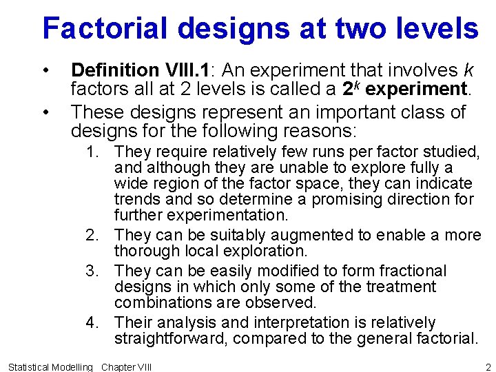
Factorial designs at two levels • • Definition VIII. 1: An experiment that involves k factors all at 2 levels is called a 2 k experiment. These designs represent an important class of designs for the following reasons: 1. They require relatively few runs per factor studied, and although they are unable to explore fully a wide region of the factor space, they can indicate trends and so determine a promising direction for further experimentation. 2. They can be suitably augmented to enable a more thorough local exploration. 3. They can be easily modified to form fractional designs in which only some of the treatment combinations are observed. 4. Their analysis and interpretation is relatively straightforward, compared to the general factorial. Statistical Modelling Chapter VIII 2

VIII. A Replicated 2 k experiments • An experiment involving three factors — a 23 experiment — will be used to illustrate. a)Design of replicated 2 k experiments, including R expressions • The design of this type of experiment is same as general case outlined in VII. A, Design of factorial experiments. • However, the levels used for the factors are specific to these two-level experiments. Statistical Modelling Chapter VIII 3

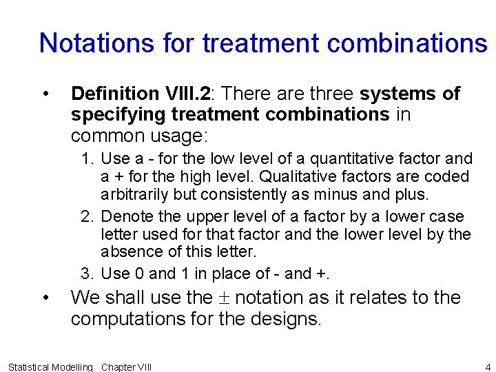
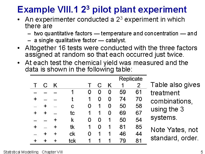
Notations for treatment combinations • Definition VIII. 2: There are three systems of specifying treatment combinations in common usage: 1. Use a - for the low level of a quantitative factor and a + for the high level. Qualitative factors are coded arbitrarily but consistently as minus and plus. 2. Denote the upper level of a factor by a lower case letter used for that factor and the lower level by the absence of this letter. 3. Use 0 and 1 in place of - and +. • We shall use the notation as it relates to the computations for the designs. Statistical Modelling Chapter VIII 4

Example VIII. 1 23 pilot plant experiment • An experimenter conducted a 23 experiment in which there are – two quantitative factors — temperature and concentration — and – a single qualitative factor — catalyst. • Altogether 16 tests were conducted with the three factors assigned at random so that each occurred just twice. • At each test the chemical yield was measured and the data is shown in the following table: Table also gives treatment combinations, using the 3 systems. Note Yates, not standard, order. Statistical Modelling Chapter VIII 5

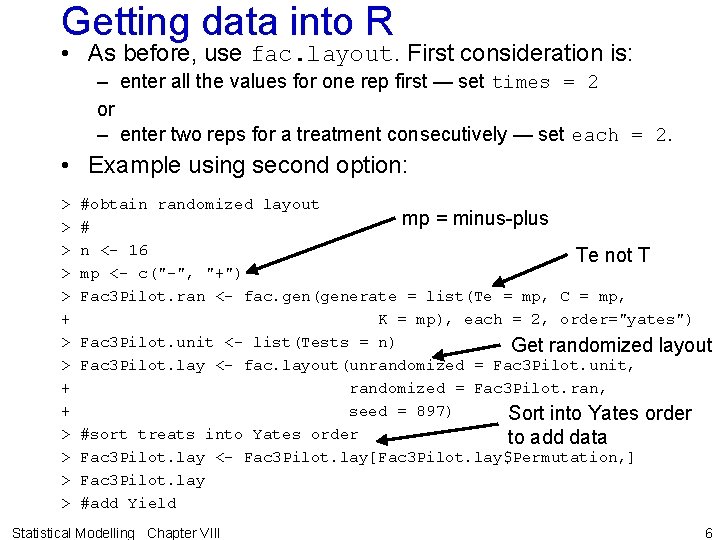
Getting data into R • As before, use fac. layout. First consideration is: – enter all the values for one rep first — set times = 2 or – enter two reps for a treatment consecutively — set each = 2. • Example using second option: > > > + + > > #obtain randomized layout mp = minus-plus # n <- 16 Te not T mp <- c("-", "+") Fac 3 Pilot. ran <- fac. gen(generate = list(Te = mp, C = mp, K = mp), each = 2, order="yates") Fac 3 Pilot. unit <- list(Tests = n) Get randomized layout Fac 3 Pilot. lay <- fac. layout(unrandomized = Fac 3 Pilot. unit, randomized = Fac 3 Pilot. ran, seed = 897) Sort into Yates order #sort treats into Yates order to add data Fac 3 Pilot. lay <- Fac 3 Pilot. lay[Fac 3 Pilot. lay$Permutation, ] Fac 3 Pilot. lay #add Yield Statistical Modelling Chapter VIII 6

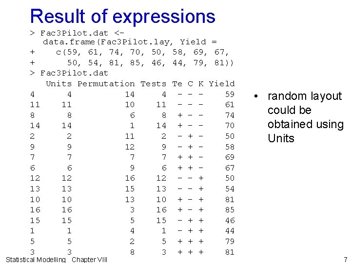
Result of expressions > Fac 3 Pilot. dat <data. frame(Fac 3 Pilot. lay, Yield = + c(59, 61, 74, 70, 58, 69, 67, + 50, 54, 81, 85, 46, 44, 79, 81)) > Fac 3 Pilot. dat Units Permutation Tests Te C K Yield 4 4 14 4 - - 59 11 11 10 11 - - 61 8 8 6 8 + - 74 14 14 1 14 + - 70 2 2 11 2 - + 50 9 9 12 9 - + 58 7 7 + + 69 6 6 9 6 + + 67 12 12 16 12 - - + 50 13 13 15 13 - - + 54 10 10 13 10 + - + 81 16 16 3 16 + - + 85 15 15 - + + 46 1 1 4 1 - + + 44 5 5 2 5 + + + 79 3 3 8 3 + + + 81 Statistical Modelling Chapter VIII • random layout could be obtained using Units 7

b) Analysis of variance • The analysis of replicated 2 k factorial experiments is the same as for the general factorial experiment. Statistical Modelling Chapter VIII 8

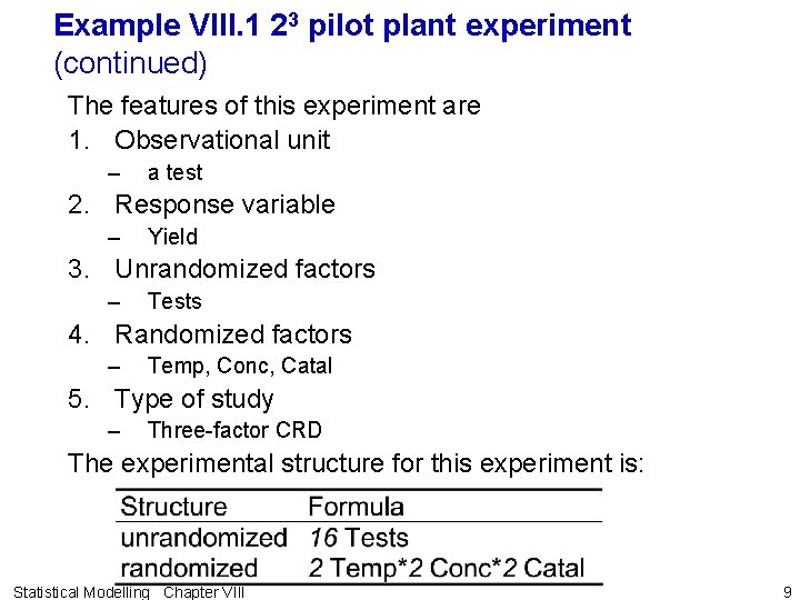
Example VIII. 1 23 pilot plant experiment (continued) The features of this experiment are 1. Observational unit – a test 2. Response variable – Yield 3. Unrandomized factors – Tests 4. Randomized factors – Temp, Conc, Catal 5. Type of study – Three-factor CRD The experimental structure for this experiment is: Statistical Modelling Chapter VIII 9

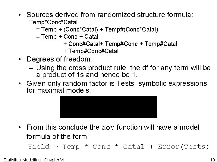
• Sources derived from randomized structure formula: Temp*Conc*Catal = Temp + (Conc*Catal) + Temp#(Conc*Catal) = Temp + Conc + Catal + Conc#Catal+ Temp#Conc + Temp#Catal + Temp#Conc#Catal • Degrees of freedom – Using the cross product rule, the df for any term will be a product of 1 s and hence be 1. • Given only random factor is Tests, symbolic expressions for maximal models: • From this conclude the aov function will have a model formula of the form Yield ~ Temp * Conc * Catal + Error(Tests) Statistical Modelling Chapter VIII 10

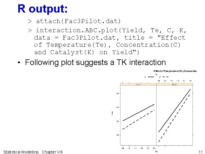
R output: > attach(Fac 3 Pilot. dat) > interaction. ABC. plot(Yield, Te, C, K, data = Fac 3 Pilot. dat, title = "Effect of Temperature(Te), Concentration(C) and Catalyst(K) on Yield") • Following plot suggests a TK interaction Statistical Modelling Chapter VIII 11

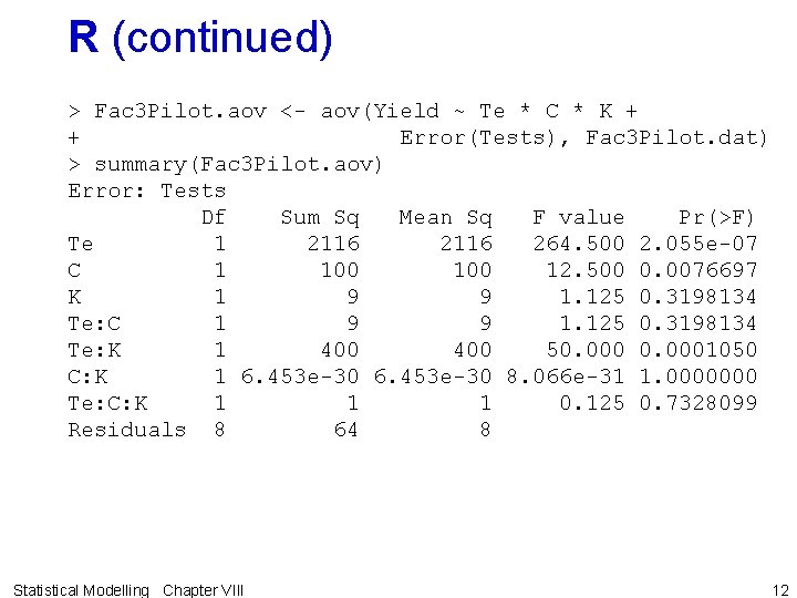
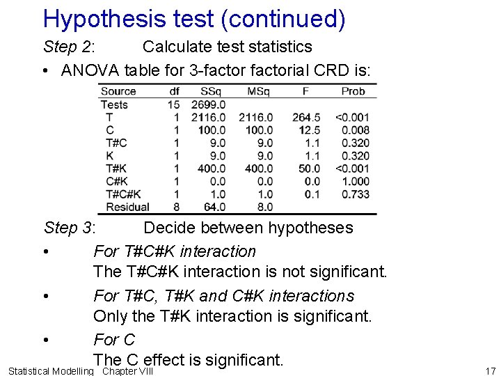
R (continued) > Fac 3 Pilot. aov <- aov(Yield ~ Te * C * K + + Error(Tests), Fac 3 Pilot. dat) > summary(Fac 3 Pilot. aov) Error: Tests Df Sum Sq Mean Sq F value Pr(>F) Te 1 2116 264. 500 2. 055 e-07 C 1 100 12. 500 0. 0076697 K 1 9 9 1. 125 0. 3198134 Te: C 1 9 9 1. 125 0. 3198134 Te: K 1 400 50. 0001050 C: K 1 6. 453 e-30 8. 066 e-31 1. 0000000 Te: C: K 1 1 1 0. 125 0. 7328099 Residuals 8 64 8 Statistical Modelling Chapter VIII 12

R output (continued) > > > # # Diagnostic checking # res <- resid. errors(Fac 3 Pilot. aov) fit <- fitted. errors(Fac 3 Pilot. aov) plot(fit, res, pch=16) plot(as. numeric(Te), res, pch=16) plot(as. numeric(C), res, pch=16) plot(as. numeric(K), res, pch=16) qqnorm(res, pch=16) qqline(res) • Note, because no additive expectation terms, instructions for Tukey's one-degree-of-freedom -for-nonadditivity not included. Statistical Modelling Chapter VIII 13

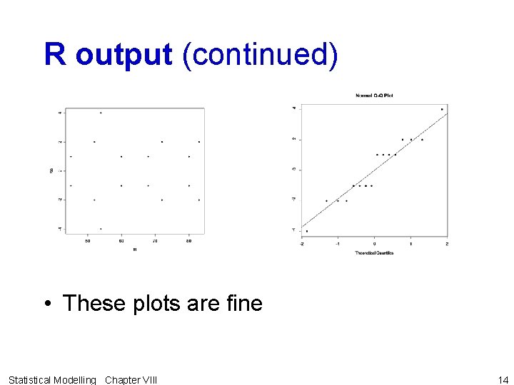
R output (continued) • These plots are fine Statistical Modelling Chapter VIII 14

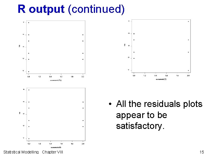
R output (continued) • All the residuals plots appear to be satisfactory. Statistical Modelling Chapter VIII 15

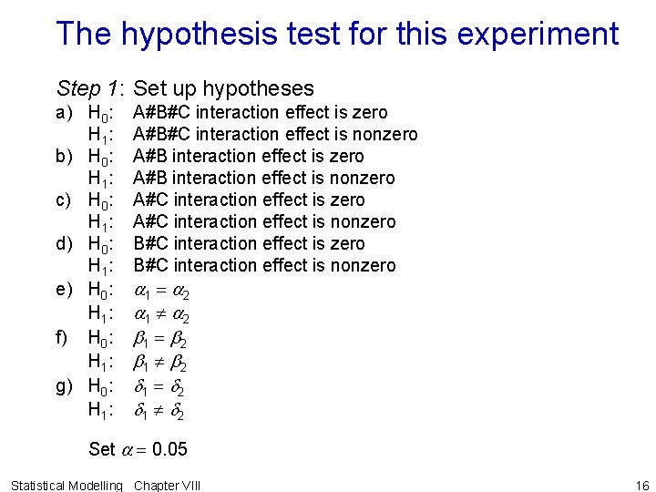
The hypothesis test for this experiment Step 1: Set up hypotheses a) H 0: H 1 : b) H 0: H 1 : c) H 0: H 1 : d) H 0: H 1 : e) H 0: H 1 : f) H 0: H 1 : g) H 0: H 1 : A#B#C interaction effect is zero A#B#C interaction effect is nonzero A#B interaction effect is nonzero A#C interaction effect is nonzero B#C interaction effect is nonzero a 1 = a 2 a 1 a 2 b 1 = b 2 b 1 b 2 d 1 = d 2 d 1 d 2 Set a = 0. 05 Statistical Modelling Chapter VIII 16

Hypothesis test (continued) Step 2: Calculate test statistics • ANOVA table for 3 -factorial CRD is: Step 3: Decide between hypotheses • For T#C#K interaction The T#C#K interaction is not significant. • For T#C, T#K and C#K interactions Only the T#K interaction is significant. • For C The C effect is significant. Statistical Modelling Chapter VIII 17

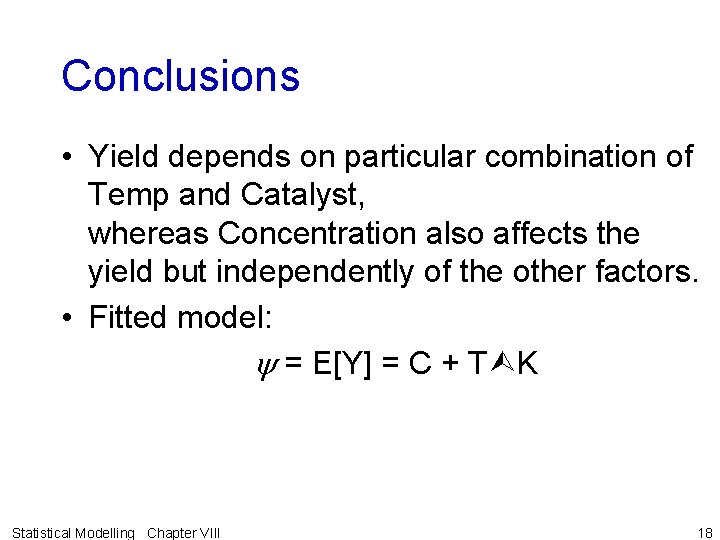
Conclusions • Yield depends on particular combination of Temp and Catalyst, whereas Concentration also affects the yield but independently of the other factors. • Fitted model: y = E[Y] = C + T K Statistical Modelling Chapter VIII 18

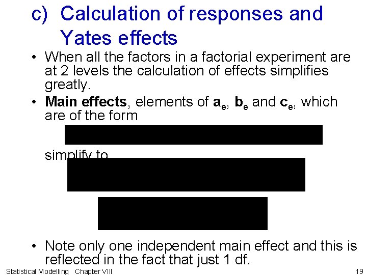
c) Calculation of responses and Yates effects • When all the factors in a factorial experiment are at 2 levels the calculation of effects simplifies greatly. • Main effects, elements of ae, be and ce, which are of the form simplify to • Note only one independent main effect and this is reflected in the fact that just 1 df. Statistical Modelling Chapter VIII 19

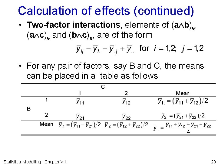
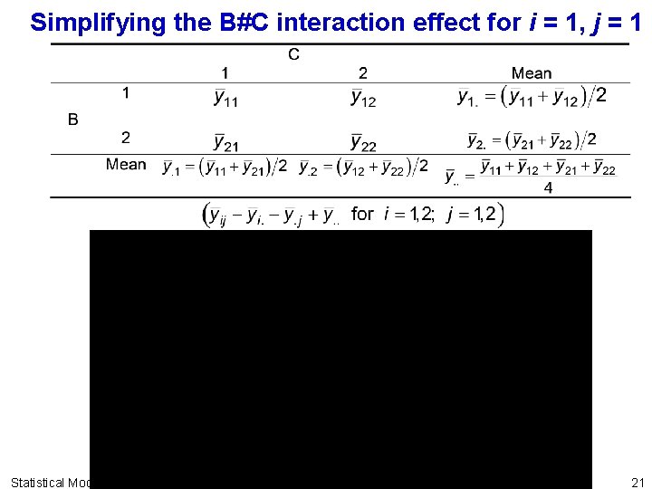
Calculation of effects (continued) • Two-factor interactions, elements of (a b)e, (a c)e and (b c)e, are of the form • For any pair of factors, say B and C, the means can be placed in a table as follows. Statistical Modelling Chapter VIII 20

Simplifying the B#C interaction effect for i = 1, j = 1 Statistical Modelling Chapter VIII 21

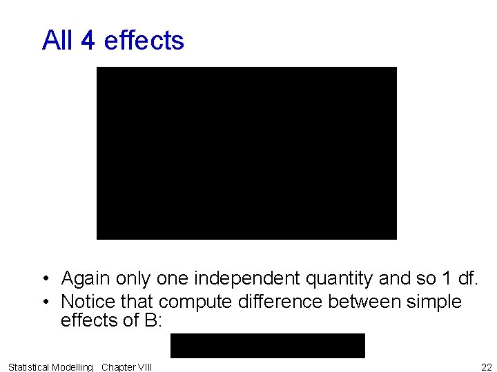
All 4 effects • Again only one independent quantity and so 1 df. • Notice that compute difference between simple effects of B: Statistical Modelling Chapter VIII 22

Calculation of effects (continued) • All effects in a 2 k experiment have only 1 df. • So to accomplish an analysis we actually only need to compute a single value for each effect, instead of a vector of effects. – We compute what are called the responses and, from these, the Yates main and interaction effects. – Not exactly the quantities above, but proportional to them. Statistical Modelling Chapter VIII 23

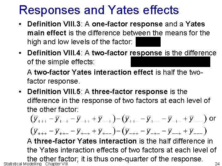
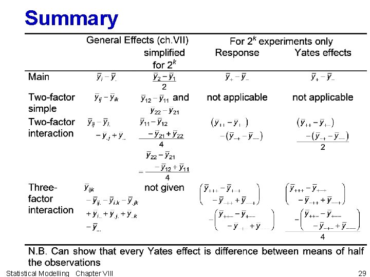
Responses and Yates effects • Definition VIII. 3: A one-factor response and a Yates main effect is the difference between the means for the high and low levels of the factor: • Definition VIII. 4: A two-factor response is the difference of the simple effects: A two-factor Yates interaction effect is half the twofactor response. • Definition VIII. 5: A three-factor response is the difference in the response of two factors at each level of the other factor: A three-factor Yates interaction is the half difference in the Yates interaction effects of two factors at each level of the other factor; it is thus one-quarter of the response. Statistical Modelling Chapter VIII 24

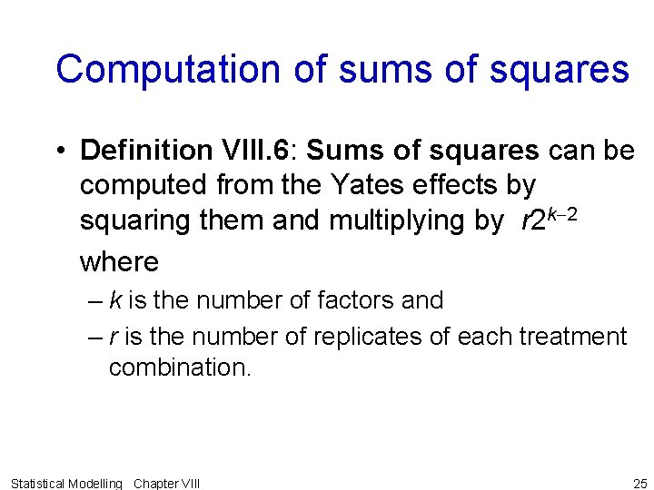
Computation of sums of squares • Definition VIII. 6: Sums of squares can be computed from the Yates effects by squaring them and multiplying by r 2 k-2 where – k is the number of factors and – r is the number of replicates of each treatment combination. Statistical Modelling Chapter VIII 25

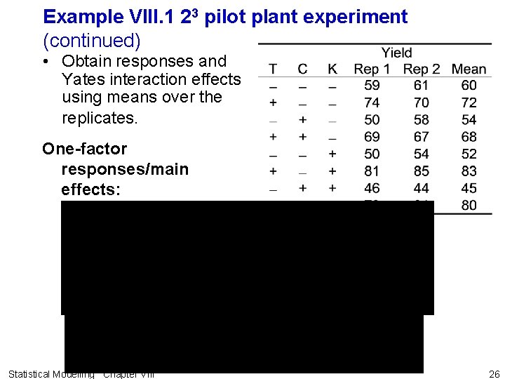
Example VIII. 1 23 pilot plant experiment (continued) • Obtain responses and Yates interaction effects using means over the replicates. One-factor responses/main effects: Statistical Modelling Chapter VIII 26

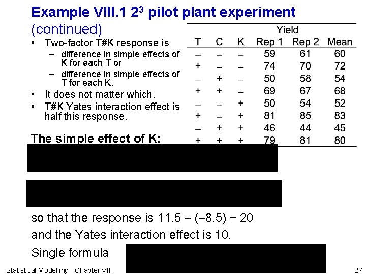
Example VIII. 1 23 pilot plant experiment (continued) • Two-factor T#K response is – difference in simple effects of K for each T or – difference in simple effects of T for each K. • It does not matter which. • T#K Yates interaction effect is half this response. The simple effect of K: so that the response is 11. 5 - (-8. 5) = 20 and the Yates interaction effect is 10. Single formula Statistical Modelling Chapter VIII 27

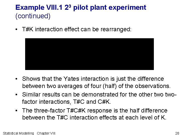
Example VIII. 1 23 pilot plant experiment (continued) • T#K interaction effect can be rearranged: • Shows that the Yates interaction is just the difference between two averages of four (half) of the observations. • Similar results can be demonstrated for the other twofactor interactions, T#C and C#K. • The three-factor T#C#K response is the half difference between the T#C interaction effects at each level of K. Statistical Modelling Chapter VIII 28

Summary Statistical Modelling Chapter VIII 29

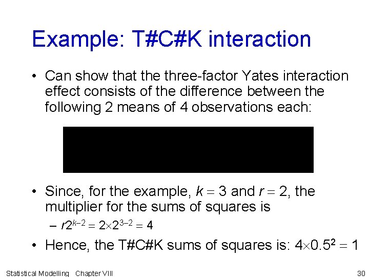
Example: T#C#K interaction • Can show that the three-factor Yates interaction effect consists of the difference between the following 2 means of 4 observations each: • Since, for the example, k = 3 and r = 2, the multiplier for the sums of squares is – r 2 k-2 = 2 23 -2 = 4 • Hence, the T#C#K sums of squares is: 4 0. 52 = 1 Statistical Modelling Chapter VIII 30

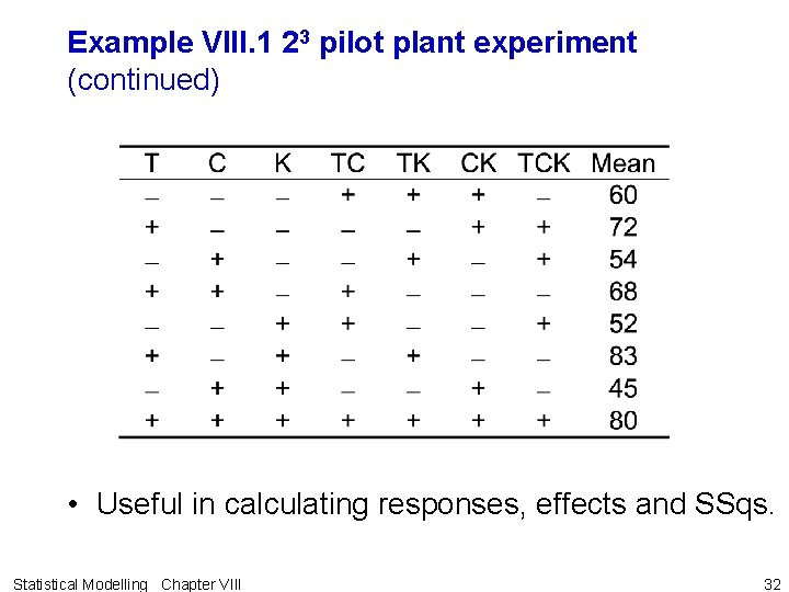
Easy rules for determining the signs of observations to compute the Yates effects • Definition VIII. 7: The signs for observations in a Yates effect are obtained from the columns of pluses and minuses that specify the factor combinations for each observation by – taking the columns for the factors in the effect and forming their elementwise product. • The elementwise product is the result of multiplying pairs of elements in the same row as if they were ± 1 and expressing the result as a ±. Statistical Modelling Chapter VIII 31

Example VIII. 1 23 pilot plant experiment (continued) • Useful in calculating responses, effects and SSqs. Statistical Modelling Chapter VIII 32

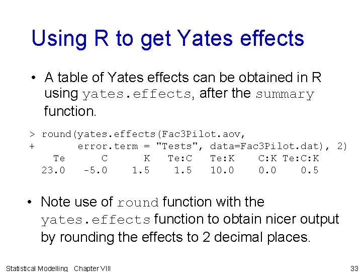
Using R to get Yates effects • A table of Yates effects can be obtained in R using yates. effects, after the summary function. > round(yates. effects(Fac 3 Pilot. aov, + error. term = "Tests", data=Fac 3 Pilot. dat), 2) Te C K Te: C Te: K C: K Te: C: K 23. 0 -5. 0 1. 5 10. 0 0. 5 • Note use of round function with the yates. effects function to obtain nicer output by rounding the effects to 2 decimal places. Statistical Modelling Chapter VIII 33

d) Yates algorithm • See notes Statistical Modelling Chapter VIII 34

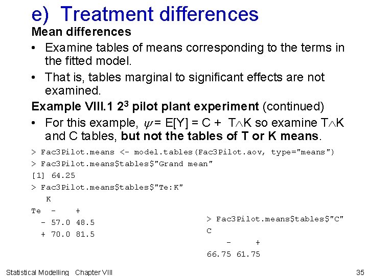
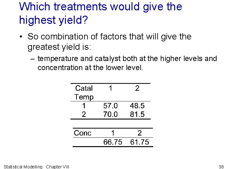
e) Treatment differences Mean differences • Examine tables of means corresponding to the terms in the fitted model. • That is, tables marginal to significant effects are not examined. Example VIII. 1 23 pilot plant experiment (continued) • For this example, y = E[Y] = C + T K so examine T K and C tables, but not the tables of T or K means. > Fac 3 Pilot. means <- model. tables(Fac 3 Pilot. aov, type="means") > Fac 3 Pilot. means$tables$"Grand mean" [1] 64. 25 > Fac 3 Pilot. means$tables$"Te: K" K Te + > Fac 3 Pilot. means$tables$"C" - 57. 0 48. 5 C + 70. 0 81. 5 + 66. 75 61. 75 Statistical Modelling Chapter VIII 35

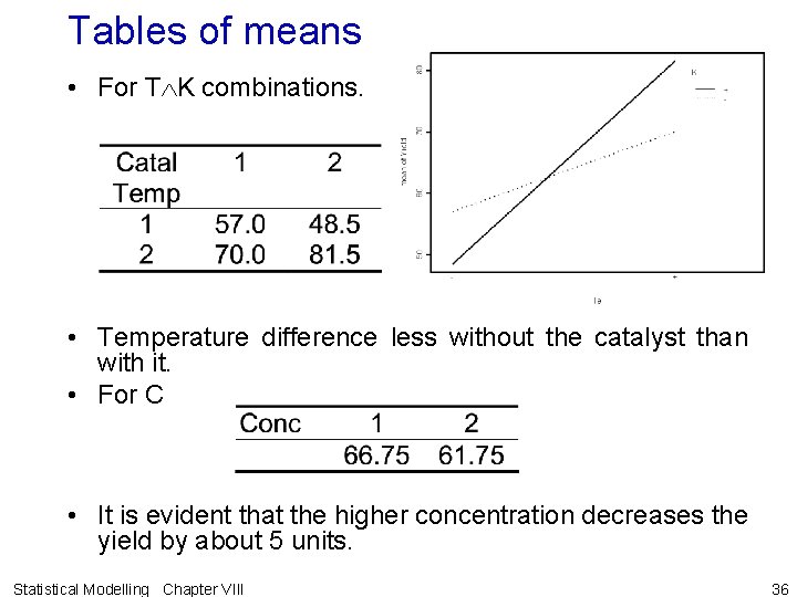
Tables of means • For T K combinations. • Temperature difference less without the catalyst than with it. • For C • It is evident that the higher concentration decreases the yield by about 5 units. Statistical Modelling Chapter VIII 36

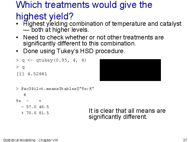
Which treatments would give the highest yield? • Highest yielding combination of temperature and catalyst — both at higher levels. • Need to check whether or not other treatments are significantly different to this combination. • Done using Tukey’s HSD procedure. > q <- qtukey(0. 95, 4, 8) > q [1] 4. 52881 > Fac 3 Pilot. means$tables$"Te: K" K Te + - 57. 0 48. 5 It is clear that all means are + 70. 0 81. 5 significantly different. Statistical Modelling Chapter VIII 37

Which treatments would give the highest yield? • So combination of factors that will give the greatest yield is: – temperature and catalyst both at the higher levels and concentration at the lower level. Statistical Modelling Chapter VIII 38

Polynomial models and fitted values • As only 2 levels of each factor, a linear trend would fit perfectly the means of each factor. • Could fit polynomial model with – the values of the factor levels for each factor as a column in an X matrix; – a linear interaction term fitted by adding to X a column that is the product of columns for the factors involved in the interaction. • However, suppose decided to code the values in X as ± 1. – Interaction terms can still be fitted as the pairwise products of the (coded) elements from the columns for the factors involved in the interaction. • X matrix, with 0, 1 or ± 1 s or the actual factor values, – give equivalent fits as fitted values and F test statistics will be the same for all three parametrizations. – Values of the parameter estimates will differ and you will need to put in the values you used in the X matrix to obtain the estimates. – The advantage of using ± 1 is the ease of obtaining the X matrix and the simplicity of the computations. – The columns of an X for a particular model obtained from the table of coefficients, with a column added for the grand mean term. Statistical Modelling Chapter VIII 39

Fitted values for X with ± 1 Definition VIII. 8: The fitted values are obtained using the fitted equation that consists of the grand mean, the xterm for each significant effect and those for effects of lower degree than the significant sources. • An x-term consists of the product of x variables, one for each factor in the term; the x variables take the values -1 and +1 according whether the fitted value is required for an observation that received the low or high level of that factor. • The coefficient of the term is half the Yates main or interaction effect. • The columns of an X for a particular model obtained from the table of coefficients, with a column added for the grand mean term. Statistical Modelling Chapter VIII 40

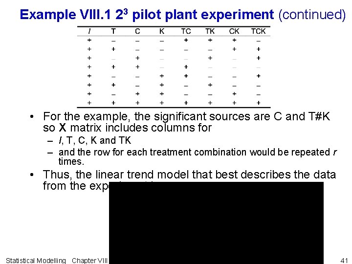
Example VIII. 1 23 pilot plant experiment (continued) • For the example, the significant sources are C and T#K so X matrix includes columns for – I, T, C, K and TK – and the row for each treatment combination would be repeated r times. • Thus, the linear trend model that best describes the data from the experiment is: Statistical Modelling Chapter VIII 41

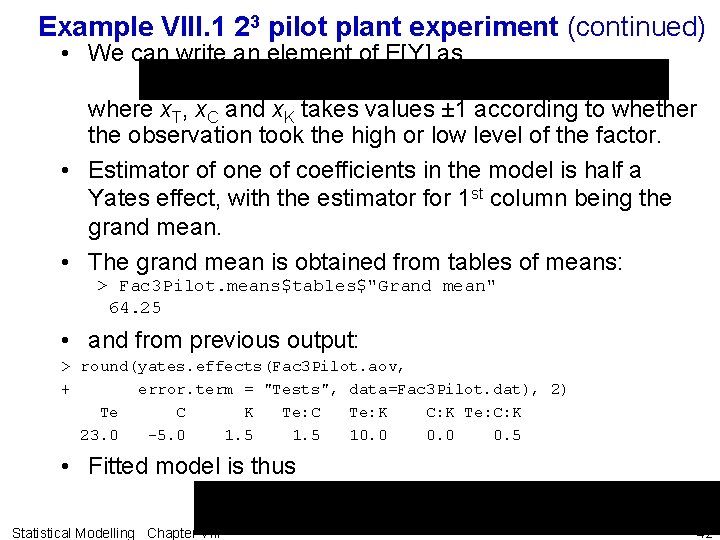
Example VIII. 1 23 pilot plant experiment (continued) • We can write an element of E[Y] as where x. T, x. C and x. K takes values ± 1 according to whether the observation took the high or low level of the factor. • Estimator of one of coefficients in the model is half a Yates effect, with the estimator for 1 st column being the grand mean. • The grand mean is obtained from tables of means: > Fac 3 Pilot. means$tables$"Grand mean" 64. 25 • and from previous output: > round(yates. effects(Fac 3 Pilot. aov, + error. term = "Tests", data=Fac 3 Pilot. dat), 2) Te C K Te: C Te: K C: K Te: C: K 23. 0 -5. 0 1. 5 10. 0 0. 5 • Fitted model is thus Statistical Modelling Chapter VIII 42

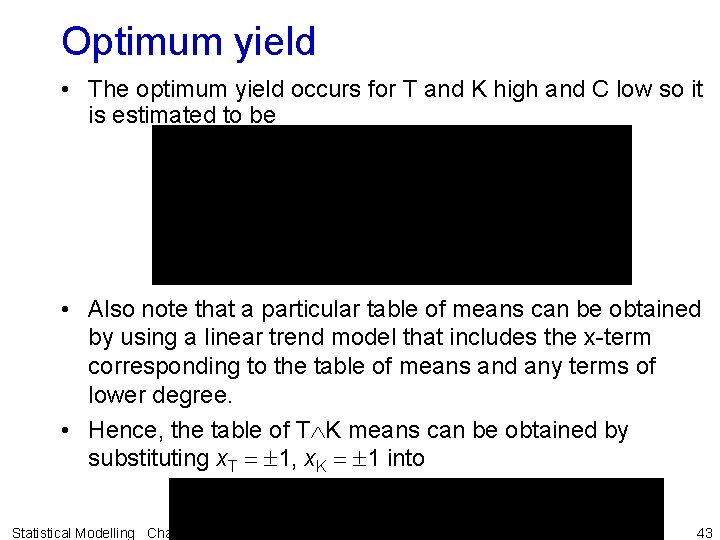
Optimum yield • The optimum yield occurs for T and K high and C low so it is estimated to be • Also note that a particular table of means can be obtained by using a linear trend model that includes the x-term corresponding to the table of means and any terms of lower degree. • Hence, the table of T K means can be obtained by substituting x. T = 1, x. K = 1 into Statistical Modelling Chapter VIII 43

VIII. B Economy in experimentation • Run 2 k experiments unreplicated. • Apparent problem: cannot measure uncontrolled variation. • However, when there are 4 or more factors it is unlikely that all factors will affect the response. • Further it is usual that the magnitudes of effects are getting smaller as the order of the effect increases. • Thus, likely that 3 -factor and higher-order interactions will be small and can be ignored without seriously affecting the conclusions drawn from the experiment. Statistical Modelling Chapter VIII 44

a) Design of unreplicated 2 k experiments, including R expressions • As there is only a single replicate, these combinations will be completely randomized to the available units. • No. units must equal total number of treatment combinations, 2 k. • To generate a design in R, – use fac. gen to generate the treatment combinations in Yates order – then fac. layout with the expressions for a CRD to randomize it. Statistical Modelling Chapter VIII 45

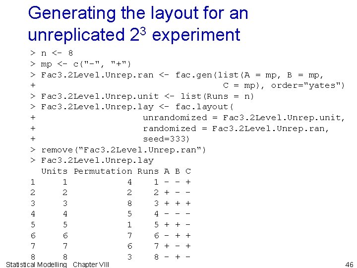
Generating the layout for an unreplicated 23 experiment > > > + + + > > 1 2 3 4 5 6 7 8 n <- 8 mp <- c("-", "+") Fac 3. 2 Level. Unrep. ran <- fac. gen(list(A = mp, B = mp, C = mp), order="yates") Fac 3. 2 Level. Unrep. unit <- list(Runs = n) Fac 3. 2 Level. Unrep. lay <- fac. layout( unrandomized = Fac 3. 2 Level. Unrep. unit, randomized = Fac 3. 2 Level. Unrep. ran, seed=333) remove("Fac 3. 2 Level. Unrep. ran") Fac 3. 2 Level. Unrep. lay Units Permutation Runs A B C 1 4 1 - - + 2 2 2 + - 3 8 3 + + + 4 5 4 - - 5 1 5 + + 6 7 6 - + + 7 6 7 + - + 8 3 8 - + - Statistical Modelling Chapter VIII 46

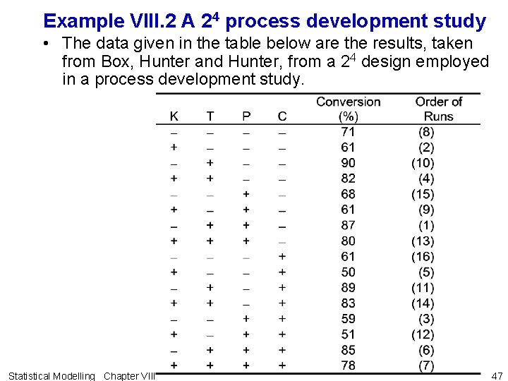
Example VIII. 2 A 24 process development study • The data given in the table below are the results, taken from Box, Hunter and Hunter, from a 24 design employed in a process development study. Statistical Modelling Chapter VIII 47

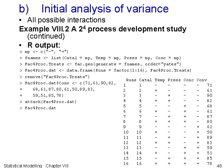
b) Initial analysis of variance • All possible interactions Example VIII. 2 A 24 process development study (continued) • R output: > > > + + > > mp <- c("-", "+") fnames <- list(Catal = mp, Temp = mp, Press = mp, Conc = mp) Fac 4 Proc. Treats <- fac. gen(generate = fnames, order="yates") Fac 4 Proc. dat <- data. frame(Runs = factor(1: 16), Fac 4 Proc. Treats) remove("Fac 4 Proc. Treats") Runs Catal Temp Press Conc Fac 4 Proc. dat$Conv <- c(71, 61, 90, 82, 1 1 68, 61, 87, 80, 61, 50, 89, 83, 2 2 + 59, 51, 85, 78) 3 3 + 4 4 + + attach(Fac 4 Proc. dat) 5 5 + Fac 4 Proc. dat 6 6 + + 7 7 + + 8 8 + + + 9 9 10 10 + 11 11 + 12 12 + + 13 13 + 14 14 + + 15 15 + + 16 16 + + + Statistical Modelling Chapter VIII Conv 71 61 90 82 68 61 87 80 + 61 + 50 + 89 + 83 + 59 + 51 + 85 + 78 48

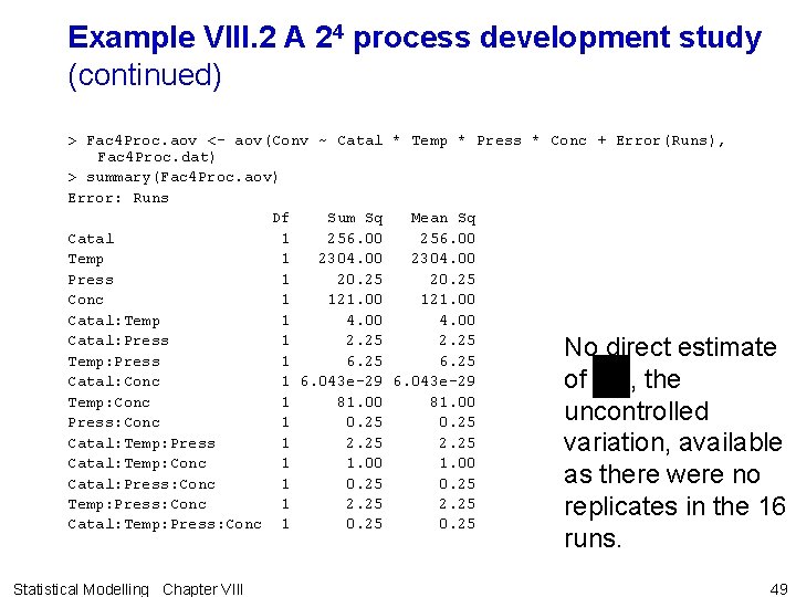
Example VIII. 2 A 24 process development study (continued) > Fac 4 Proc. aov <- aov(Conv ~ Catal * Temp * Press * Conc + Error(Runs), Fac 4 Proc. dat) > summary(Fac 4 Proc. aov) Error: Runs Df Sum Sq Mean Sq Catal 1 256. 00 Temp 1 2304. 00 Press 1 20. 25 Conc 1 121. 00 Catal: Temp 1 4. 00 Catal: Press 1 2. 25 Temp: Press 1 6. 25 Catal: Conc 1 6. 043 e-29 Temp: Conc 1 81. 00 Press: Conc 1 0. 25 Catal: Temp: Press 1 2. 25 Catal: Temp: Conc 1 1. 00 Catal: Press: Conc 1 0. 25 Temp: Press: Conc 1 2. 25 Catal: Temp: Press: Conc 1 0. 25 No direct estimate of , the uncontrolled variation, available as there were no replicates in the 16 runs. Statistical Modelling Chapter VIII 49

c) Analysis assuming no 3 -factor or 4 -factor interactions • However, if we assume that all three-factor and four-factor interactions are negligible, – then we could use these to estimate the uncontrolled variation as this is the only reason for them being nonzero. • To do this rerun the analysis with the model consisting of a list of factors separated by pluses and raised to the power 2. Statistical Modelling Chapter VIII 50

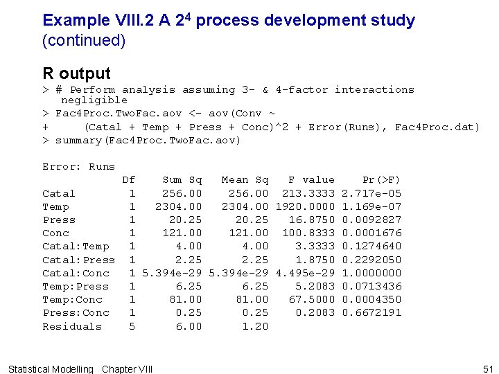
Example VIII. 2 A 24 process development study (continued) R output > # Perform analysis assuming 3 - & 4 -factor interactions negligible > Fac 4 Proc. Two. Fac. aov <- aov(Conv ~ + (Catal + Temp + Press + Conc)^2 + Error(Runs), Fac 4 Proc. dat) > summary(Fac 4 Proc. Two. Fac. aov) Error: Runs Df Sum Sq Mean Sq F value Pr(>F) Catal 1 256. 00 213. 3333 2. 717 e-05 Temp 1 2304. 00 1920. 0000 1. 169 e-07 Press 1 20. 25 16. 8750 0. 0092827 Conc 1 121. 00 100. 8333 0. 0001676 Catal: Temp 1 4. 00 3. 3333 0. 1274640 Catal: Press 1 2. 25 1. 8750 0. 2292050 Catal: Conc 1 5. 394 e-29 4. 495 e-29 1. 0000000 Temp: Press 1 6. 25 5. 2083 0. 0713436 Temp: Conc 1 81. 00 67. 5000 0. 0004350 Press: Conc 1 0. 25 0. 2083 0. 6672191 Residuals 5 6. 00 1. 20 Statistical Modelling Chapter VIII 51

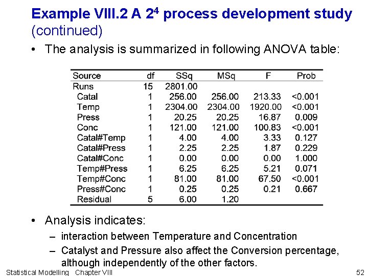
Example VIII. 2 A 24 process development study (continued) • The analysis is summarized in following ANOVA table: • Analysis indicates: – interaction between Temperature and Concentration – Catalyst and Pressure also affect the Conversion percentage, although independently of the other factors. Statistical Modelling Chapter VIII 52

Example VIII. 2 A 24 process development study (continued) • However, there is a problem with this in that – the test for main effects has been preceded by a test for interaction terms. thus, testing is not independent and an allowance needs to be made for this. – occasionally meaningful higher order interactions occur and so should not use them in the error. • The analysis presented above does not confront either of these problems. Statistical Modelling Chapter VIII 53

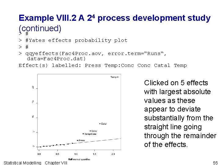
d) Probability plot of Yates effects • A method that: – does not require the assumption of zero higher-order interactions – allows for the dependence of the testing is a Normal probability plot of the Yates effects. • For the above reasons this is the preferred method, particularly for unreplicated and fractional experiments. • Yates effects are plotted against standard normal deviates. – This is done on the basis that if there were no effects of the factors, the estimated effects would be just normally distributed uncontrolled variation. – Under these circumstances a straight-line plot of normal deviates versus Yates effects is expected. • The function qqyeffects with an aov. object as the first argument produces the plot. – Label those points that you consider significant (the outliers) by clicking on them (on the side on which you want the label) and then right-click on the graph and select Stop. – A list of selected effects is produced and a regression line plotted through the origin and unselected points (nonsignificant effects). Statistical Modelling Chapter VIII 54

Example VIII. 2 A 24 process development study (continued) > #Yates effects probability plot > # > qqyeffects(Fac 4 Proc. aov, error. term="Runs“, data=Fac 4 Proc. dat) Effect(s) labelled: Press Temp: Conc Catal Temp Clicked on 5 effects with largest absolute values as these appear to deviate substantially from the straight line going through the remainder of the effects. Statistical Modelling Chapter VIII 55

Example VIII. 2 A 24 process development study (continued) • The large Yates effects correspond to – Catalyst and Temperature, Pressure, Concentration and Temperature#Concentration. > round(yates. effects(Fac 4 Proc. aov, error. term="Runs", data=Fac 4 Proc. dat), 2) Catal Temp Press -8. 00 24. 00 -2. 25 Conc Catal: Temp Catal: Press -5. 50 1. 00 0. 75 Temp: Press Catal: Conc Temp: Conc -1. 25 0. 00 4. 50 Press: Conc Catal: Temp: Press Catal: Temp: Conc -0. 25 -0. 75 0. 50 Catal: Press: Conc Temp: Press: Conc Catal: Temp: Press: Conc -0. 25 -0. 75 -0. 25 • Conclusion: – Temperature and Concentration interact in their effect on the Conversion percentage – Pressure and Catalyst each affect the response independently of any other factors. • The fitted model is y = E[Y] = Pressure + Catalyst + Temperature Concentration Statistical Modelling Chapter VIII 56

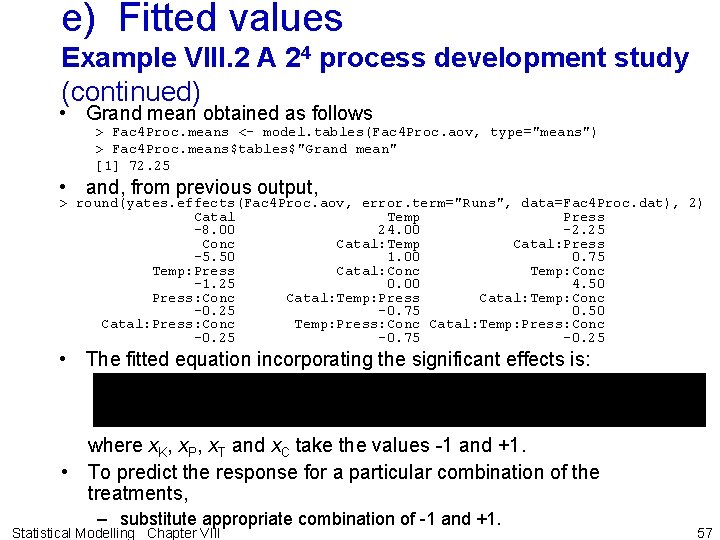
e) Fitted values Example VIII. 2 A 24 process development study (continued) • Grand mean obtained as follows > Fac 4 Proc. means <- model. tables(Fac 4 Proc. aov, type="means") > Fac 4 Proc. means$tables$"Grand mean" [1] 72. 25 • and, from previous output, > round(yates. effects(Fac 4 Proc. aov, error. term="Runs", data=Fac 4 Proc. dat), 2) Catal Temp Press -8. 00 24. 00 -2. 25 Conc Catal: Temp Catal: Press -5. 50 1. 00 0. 75 Temp: Press Catal: Conc Temp: Conc -1. 25 0. 00 4. 50 Press: Conc Catal: Temp: Press Catal: Temp: Conc -0. 25 -0. 75 0. 50 Catal: Press: Conc Temp: Press: Conc Catal: Temp: Press: Conc -0. 25 -0. 75 -0. 25 • The fitted equation incorporating the significant effects is: where x. K, x. P, x. T and x. C take the values -1 and +1. • To predict the response for a particular combination of the treatments, – substitute appropriate combination of -1 and +1. Statistical Modelling Chapter VIII 57

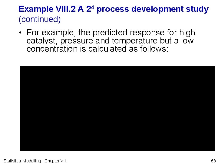
Example VIII. 2 A 24 process development study (continued) • For example, the predicted response for high catalyst, pressure and temperature but a low concentration is calculated as follows: Statistical Modelling Chapter VIII 58

f) Diagnostic checking • Having determined the significant terms, one can – reanalyze with just these terms, and those marginal to them, included in the model. formula and – obtain the Residuals from this model. • The Residuals can be used to do the usual diagnostic checking. • For this to be effective requires that – the number of fitted effects is small compared to the total number of effects in the experiment – there is at least 10 degrees of freedom for the Residual line in the analysis of variance. Statistical Modelling Chapter VIII 59

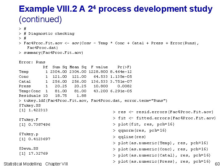
Example VIII. 2 A 24 process development study (continued) > > # # Diagnostic checking # Fac 4 Proc. Fit. aov <- aov(Conv ~ Temp * Conc + Catal + Press + Error(Runs), Fac 4 Proc. dat) > summary(Fac 4 Proc. Fit. aov) Error: Runs Df Sum Sq Mean Sq F value Pr(>F) Temp 1 2304. 00 1228. 800 8. 464 e-12 Conc 1 121. 00 64. 533 1. 135 e-05 Catal 1 256. 00 136. 533 3. 751 e-07 Press 1 20. 25 10. 800 0. 0082 Temp: Conc 1 81. 00 43. 200 6. 291 e-05 Residuals 10 18. 75 1. 88 > tukey. 1 df(Fac 4 Proc. Fit. aov, Fac 4 Proc. dat, error. term="Runs") $Tukey. SS [1] 1. 422313 > res <- resid. errors(Fac 4 Proc. Fit. aov) $Tukey. F [1] 0. 7387496 $Tukey. p [1] 0. 4123697 $Devn. SS [1] 17. 32769 Statistical Modelling Chapter VIII > > > > fit <- fitted. errors(Fac 4 Proc. Fit. aov) plot(fit, res, pch=16) qqnorm(res, pch=16) qqline(res) plot(as. numeric(Temp), res, pch=16) plot(as. numeric(Conc), res, pch=16) plot(as. numeric(Catal), res, pch=16) plot(as. numeric(Press), res, pch=16) 60

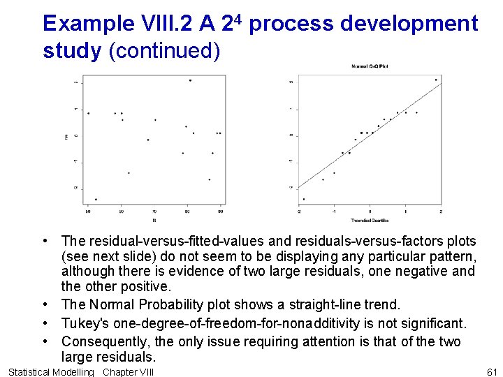
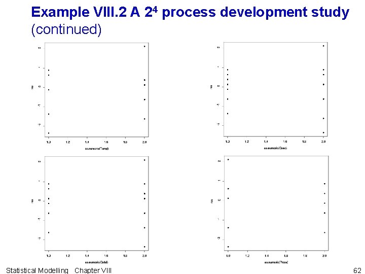
Example VIII. 2 A 24 process development study (continued) • The residual-versus-fitted-values and residuals-versus-factors plots (see next slide) do not seem to be displaying any particular pattern, although there is evidence of two large residuals, one negative and the other positive. • The Normal Probability plot shows a straight-line trend. • Tukey's one-degree-of-freedom-for-nonadditivity is not significant. • Consequently, the only issue requiring attention is that of the two large residuals. Statistical Modelling Chapter VIII 61

Example VIII. 2 A 24 process development study (continued) Statistical Modelling Chapter VIII 62

g) Treatment differences • As a result of the analysis we have – identified the model that describes the affect of the factors on the response variable and – hence the tables of means that need to be examined to determine the exact nature of the effects. Statistical Modelling Chapter VIII 63

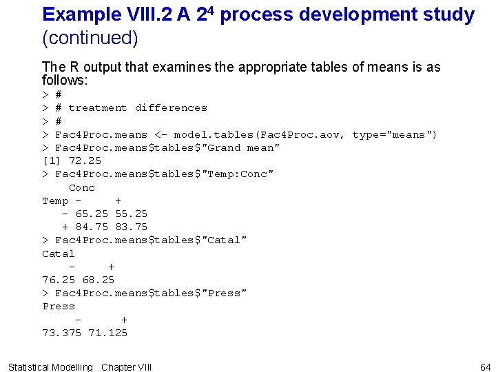
Example VIII. 2 A 24 process development study (continued) The R output that examines the appropriate tables of means is as follows: > # treatment differences > # > Fac 4 Proc. means <- model. tables(Fac 4 Proc. aov, type="means") > Fac 4 Proc. means$tables$"Grand mean" [1] 72. 25 > Fac 4 Proc. means$tables$"Temp: Conc" Conc Temp + - 65. 25 55. 25 + 84. 75 83. 75 > Fac 4 Proc. means$tables$"Catal" Catal + 76. 25 68. 25 > Fac 4 Proc. means$tables$"Press" Press + 73. 375 71. 125 Statistical Modelling Chapter VIII 64

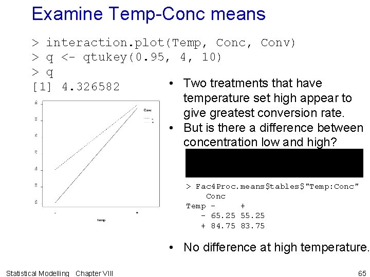
Examine Temp-Conc means > interaction. plot(Temp, Conc, Conv) > q <- qtukey(0. 95, 4, 10) > q • Two treatments that have [1] 4. 326582 temperature set high appear to give greatest conversion rate. • But is there a difference between concentration low and high? > Fac 4 Proc. means$tables$"Temp: Conc" Conc Temp + - 65. 25 55. 25 + 84. 75 83. 75 • No difference at high temperature. Statistical Modelling Chapter VIII 65

Conclusion • From the tables of means it is concluded that the maximum conversion rate will be achieved with both catalyst and pressure set low. • To achieve the maximum conversion rate, – set temperature high and set catalyst and pressure low – either setting of concentration can be used. Statistical Modelling Chapter VIII 66

VIII. C Confounding in factorial experiments a) Total confounding of effects • Not always possible to get a complete set of the treatments into a block or row. • Particular problem with factorial experiments where the number of treatments tends to be larger. • Definition VIII. 9: A confounded factorial experiment is one in which incomplete sets of treatments occur in each block. • The choice of which treatments to put in each block is done by deciding which effect is to be confounded with block differences. • Definition VIII. 10: A generator for a confounded experiment is a relationship that specifies which effect is equal to a particular block contrast. Statistical Modelling Chapter VIII 67

Example VIII. 3 Complete sets of factorial treatments in 2 blocks • Suppose that a trial is to be conducted using a 23 factorial design. • However, suppose that the available blender can only blend sufficient for four runs at a time. • This means that two blends will be required for a complete set of treatments. • Least serious thing to do is to have three factor interaction mixed up or confounded with blocks and the other effects unconfounded. Statistical Modelling Chapter VIII 68

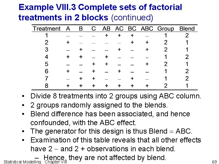
Example VIII. 3 Complete sets of factorial treatments in 2 blocks (continued) • Divide 8 treatments into 2 groups using ABC column. • 2 groups randomly assigned to the blends. • Blend difference has been associated, and hence confounded, with the ABC effect. • The generator for this design is thus Blend = ABC. • Examination of this table reveals that all other effects have 2 - and 2 + observations in each blend. – Hence, they are not affected by blend. Statistical Modelling Chapter VIII 69

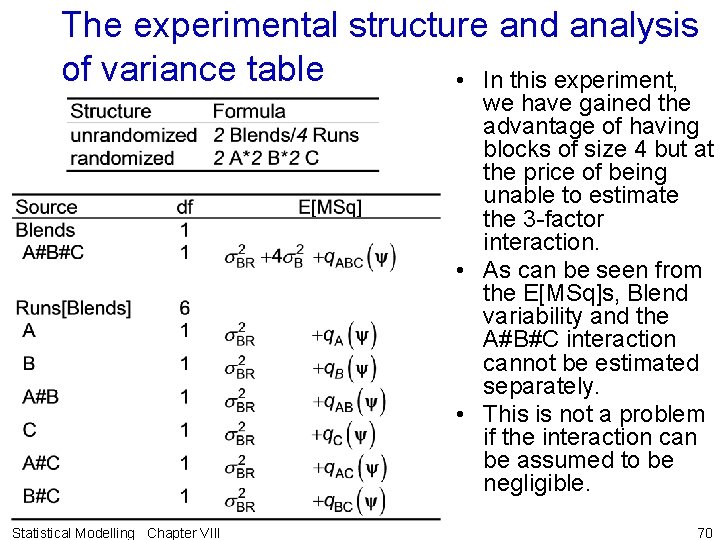
The experimental structure and analysis of variance table • In this experiment, we have gained the advantage of having blocks of size 4 but at the price of being unable to estimate the 3 -factor interaction. • As can be seen from the E[MSq]s, Blend variability and the A#B#C interaction cannot be estimated separately. • This is not a problem if the interaction can be assumed to be negligible. Statistical Modelling Chapter VIII 70

Example VIII. 4 Repeated two block experiment • To increase precision could replicate the basic design say r times which requires 2 r blends. • There is a choice as to how the 2 groups of treatments are to be assigned to the blends. • Completely randomized assignment: – groups of treatments assigned completely at random so that each group occurred with r out of the 2 r blends. • Blocked assignment: – blends are formed into blocks of two and the groups of treatments randomized to the two blends within each block; • For blocking to be worthwhile need to be able to identify relatively similar pairs of blends; • Otherwise complete randomization preferable. Statistical Modelling Chapter VIII 71

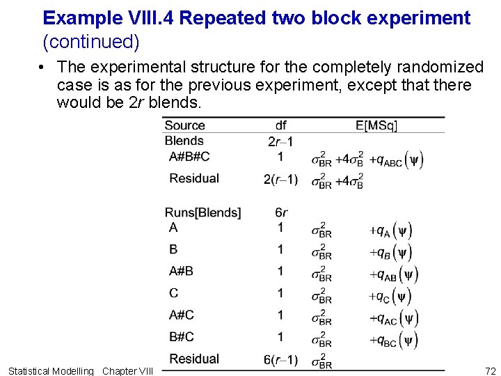
Example VIII. 4 Repeated two block experiment (continued) • The experimental structure for the completely randomized case is as for the previous experiment, except that there would be 2 r blends. Statistical Modelling Chapter VIII 72

Example VIII. 5 Complete sets of factorial treatments in 4 blocks • Suppose that a 23 experiment is to be run but that the blends are only large enough for two runs using one blend. • How can we design the experiment best? • There will be four groups of treatments which we can represent using two factors at two levels. • Let's suppose it is decided to associate the ABC interaction and one of the expendable two-factor interactions, say BC, with the blend differences. Statistical Modelling Chapter VIII 73

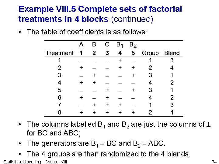
Example VIII. 5 Complete sets of factorial treatments in 4 blocks (continued) • The table of coefficients is as follows: • The columns labelled B 1 and B 2 are just the columns of for BC and ABC; • The generators are B 1 = BC and B 2 = ABC. • The 4 groups are then randomized to the 4 blends. Statistical Modelling Chapter VIII 74

Example VIII. 5 Complete sets of factorial treatments in 4 blocks (continued) • There is a serious weakness with this design!!! • There are 3 degrees of freedom associated with group differences and we know of only two degrees of freedom confounded with Blends. • What has happened to the third degree of freedom? • Well, it is obtained as the interaction of B 1 and B 2. • It will be found if you multiply these columns together you obtain the A column. • Disaster! a main effect has been confounded with Blends. Statistical Modelling Chapter VIII 75

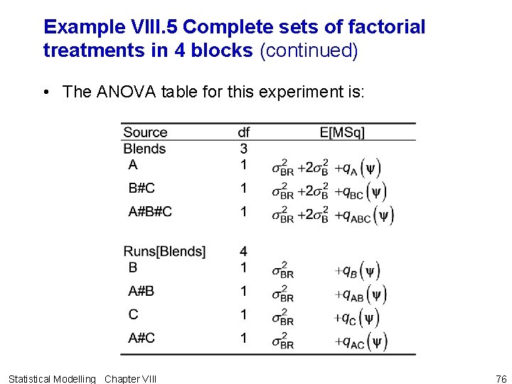
Example VIII. 5 Complete sets of factorial treatments in 4 blocks (continued) • The ANOVA table for this experiment is: Statistical Modelling Chapter VIII 76

Calculus for finding confounding • Theorem VIII. 1: Let the columns in a table of ±s whose rows specify the combinations of the factors in a two-factor experiment be numbered 1, 2, …, m. • Also, let I be the column consisting entirely of +s. • Then – the elementwise product of two columns is commutative, – the elementwise product of a column with I is the column itself and – the elementwise product of a column with itself is I. • That is, ij = ji, Ii = i. I = i and ii = I where i, j = 1, 2, …, m • Proof: follows directly from a consideration of the results of multiplying 1 s together Statistical Modelling Chapter VIII 77

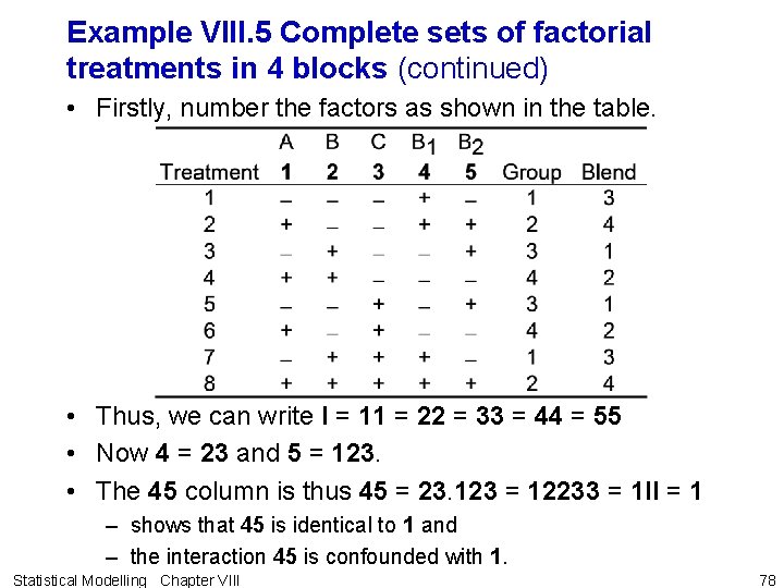
Example VIII. 5 Complete sets of factorial treatments in 4 blocks (continued) • Firstly, number the factors as shown in the table. • Thus, we can write I = 11 = 22 = 33 = 44 = 55 • Now 4 = 23 and 5 = 123. • The 45 column is thus 45 = 23. 123 = 12233 = 1 II = 1 – shows that 45 is identical to 1 and – the interaction 45 is confounded with 1. Statistical Modelling Chapter VIII 78

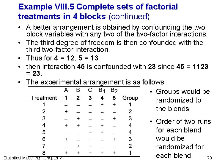
Example VIII. 5 Complete sets of factorial treatments in 4 blocks (continued) • A better arrangement is obtained by confounding the two block variables with any two of the two-factor interactions. • The third degree of freedom is then confounded with the third two-factor interaction. • Thus for 4 = 12, 5 = 13 • then interaction 45 is confounded with 23 since 45 = 1123 = 23. • The experimental arrangement is as follows: • Groups would be randomized to the blends; Statistical Modelling Chapter VIII • Order of two runs for each blend would be randomized for each blend. 79

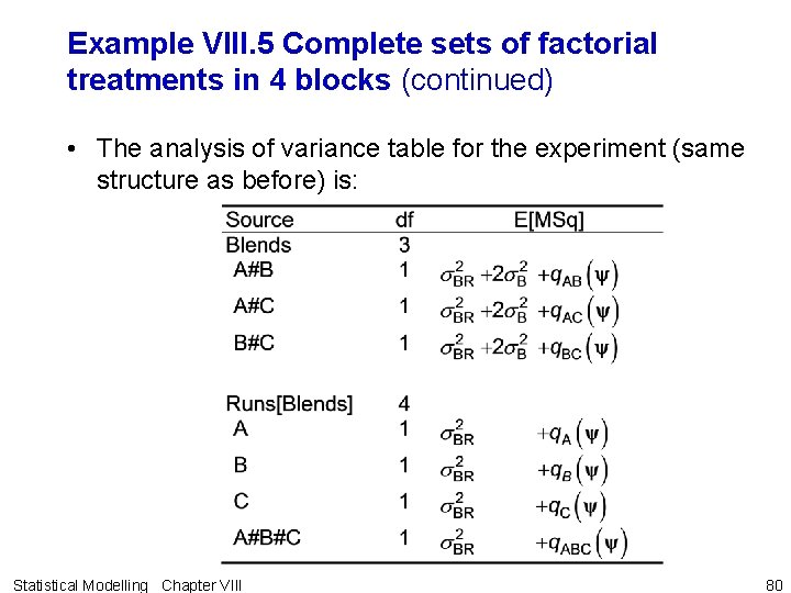
Example VIII. 5 Complete sets of factorial treatments in 4 blocks (continued) • The analysis of variance table for the experiment (same structure as before) is: Statistical Modelling Chapter VIII 80

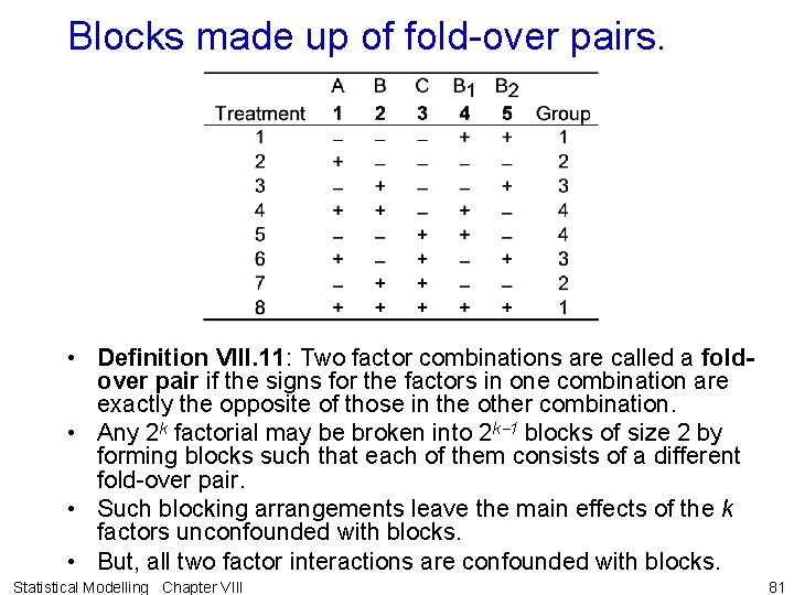
Blocks made up of fold-over pairs. • Definition VIII. 11: Two factor combinations are called a foldover pair if the signs for the factors in one combination are exactly the opposite of those in the other combination. • Any 2 k factorial may be broken into 2 k-1 blocks of size 2 by forming blocks such that each of them consists of a different fold-over pair. • Such blocking arrangements leave the main effects of the k factors unconfounded with blocks. • But, all two factor interactions are confounded with blocks. Statistical Modelling Chapter VIII 81

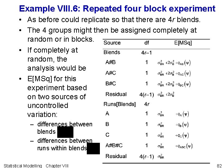
Example VIII. 6: Repeated four block experiment • As before could replicate so that there are 4 r blends. • The 4 groups might then be assigned completely at random or in blocks. • If completely at random, the analysis would be • E[MSq] for this experiment based on two sources of uncontrolled variation: – differences between blends – differences between runs within blends Statistical Modelling Chapter VIII 82

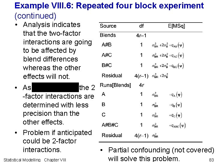
Example VIII. 6: Repeated four block experiment (continued) • Analysis indicates that the two-factor interactions are going to be affected by blend differences whereas the other effects will not. • As the 2 -factor interactions are determined with less precision than the other effects. • Problem if anticipated could be 2 -factor interactions. • Partial confounding (not covered) will solve this problem. 83 Statistical Modelling Chapter VIII

b) Partial confounding of effects • In experiments where the complete set of treatments are replicated it is possible to confound different effects in each replicate. • Definition VIII. 12: Partial confounding occurs when the effects confounded between blocks is different for different groups of blocks Statistical Modelling Chapter VIII 84

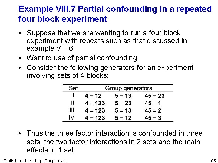
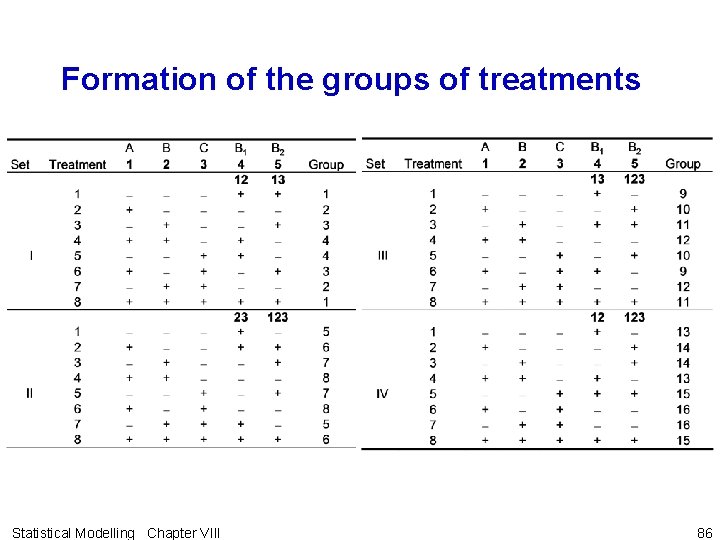
Example VIII. 7 Partial confounding in a repeated four block experiment • Suppose that we are wanting to run a four block experiment with repeats such as that discussed in example VIII. 6. • Want to use of partial confounding. • Consider the following generators for an experiment involving sets of 4 blocks: • Thus the three factor interaction is confounded in three sets, the two factor interactions in 2 sets and the main effects in 1 set. Statistical Modelling Chapter VIII 85

Formation of the groups of treatments Statistical Modelling Chapter VIII 86

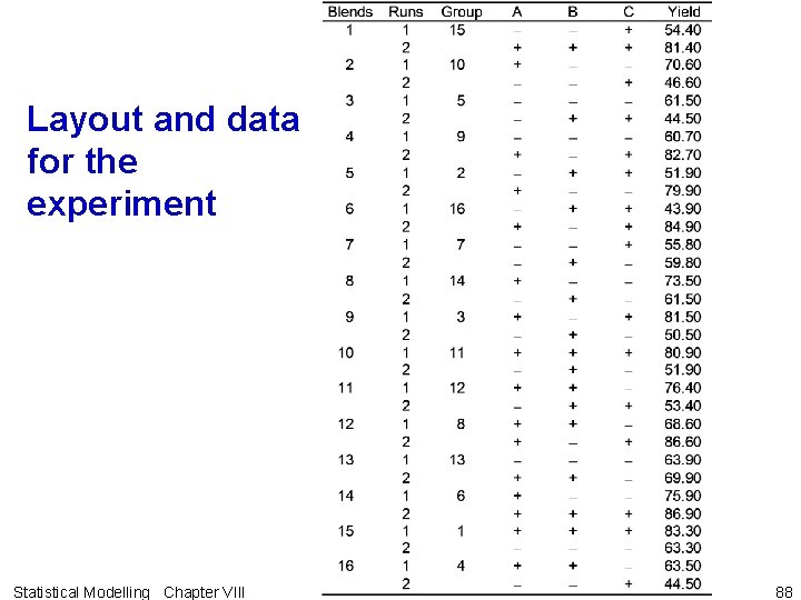
Randomization • Randomize – groups (pairs) of treatments to the blends – 2 treatment combinations in each group randomized to the 2 runs made for each blend. • A layout for such a design can be produced in R: – obtain the layout for each Set and then combine these into a single data. frame. Statistical Modelling Chapter VIII 87

Layout and data for the experiment Statistical Modelling Chapter VIII 88

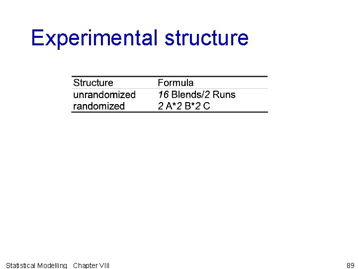
Experimental structure Statistical Modelling Chapter VIII 89

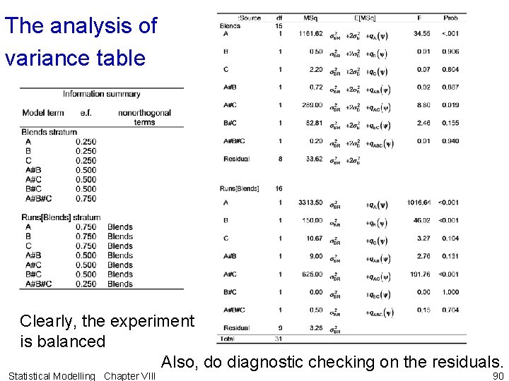
The analysis of variance table Clearly, the experiment is balanced Also, do diagnostic checking on the residuals. Statistical Modelling Chapter VIII 90

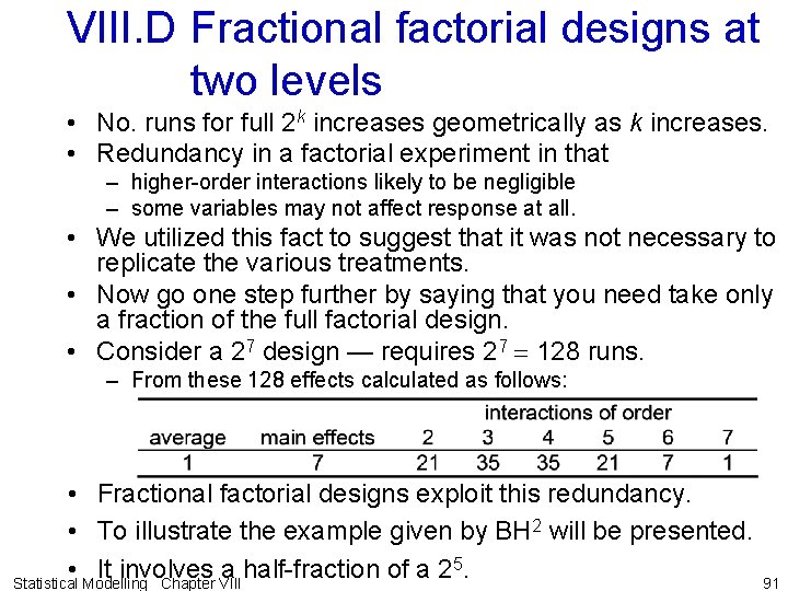
VIII. D Fractional factorial designs at two levels • No. runs for full 2 k increases geometrically as k increases. • Redundancy in a factorial experiment in that – higher-order interactions likely to be negligible – some variables may not affect response at all. • We utilized this fact to suggest that it was not necessary to replicate the various treatments. • Now go one step further by saying that you need take only a fraction of the full factorial design. • Consider a 27 design — requires 27 = 128 runs. – From these 128 effects calculated as follows: • Fractional factorial designs exploit this redundancy. • To illustrate the example given by BH 2 will be presented. 5. • It involves a half-fraction of a 2 91 Statistical Modelling Chapter VIII

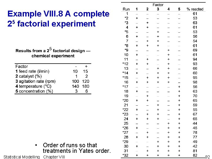
Example VIII. 8 A complete 25 factorial experiment • Order of runs so that treatments in Yates order. Statistical Modelling Chapter VIII 92

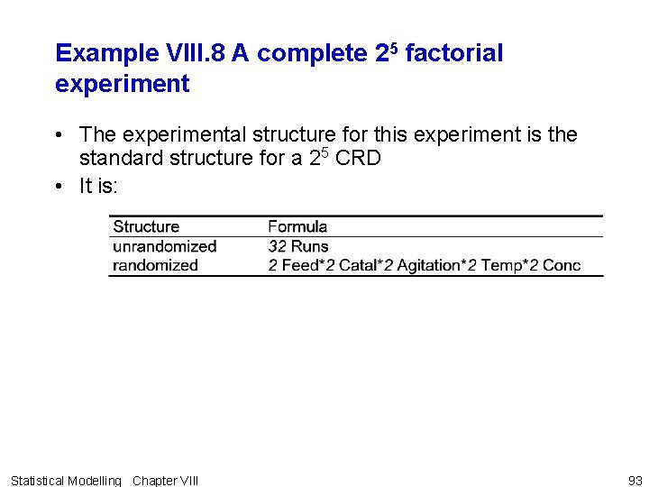
Example VIII. 8 A complete 25 factorial experiment • The experimental structure for this experiment is the standard structure for a 25 CRD • It is: Statistical Modelling Chapter VIII 93

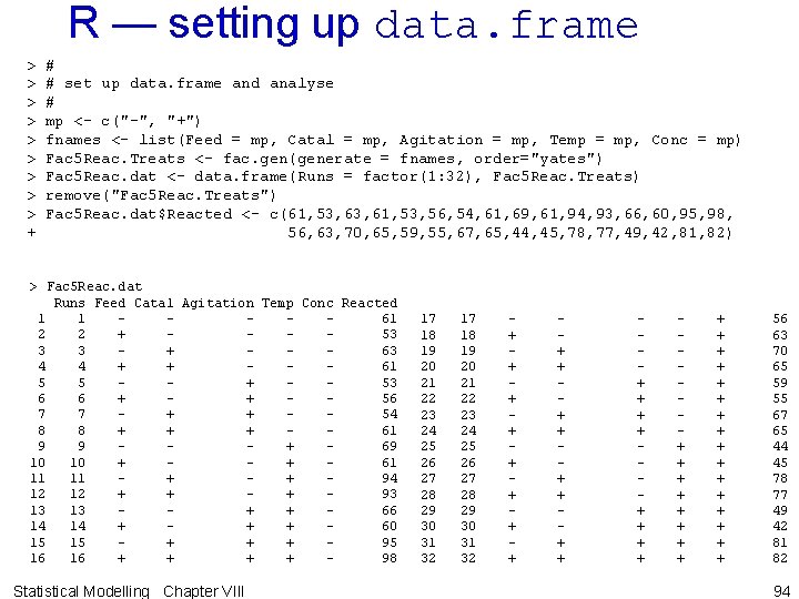
R — setting up data. frame > > > > > + # # set up data. frame and analyse # mp <- c("-", "+") fnames <- list(Feed = mp, Catal = mp, Agitation = mp, Temp = mp, Conc = mp) Fac 5 Reac. Treats <- fac. gen(generate = fnames, order="yates") Fac 5 Reac. dat <- data. frame(Runs = factor(1: 32), Fac 5 Reac. Treats) remove("Fac 5 Reac. Treats") Fac 5 Reac. dat$Reacted <- c(61, 53, 56, 54, 61, 69, 61, 94, 93, 66, 60, 95, 98, 56, 63, 70, 65, 59, 55, 67, 65, 44, 45, 78, 77, 49, 42, 81, 82) > Fac 5 Reac. dat Runs Feed Catal Agitation Temp Conc Reacted 1 1 61 2 2 + 53 3 3 + 63 4 4 + + 61 5 5 + 53 6 6 + + 56 7 7 + + 54 8 8 + + + 61 9 9 + 69 10 10 + + 61 11 11 + + 94 12 12 + + + 93 13 13 + + 66 14 14 + + + 60 15 15 + + + 95 16 16 + + 98 Statistical Modelling Chapter VIII 17 18 19 20 21 22 23 24 25 26 27 28 29 30 31 32 + + + + + + + + + + + + 56 63 70 65 59 55 67 65 44 45 78 77 49 42 81 82 94

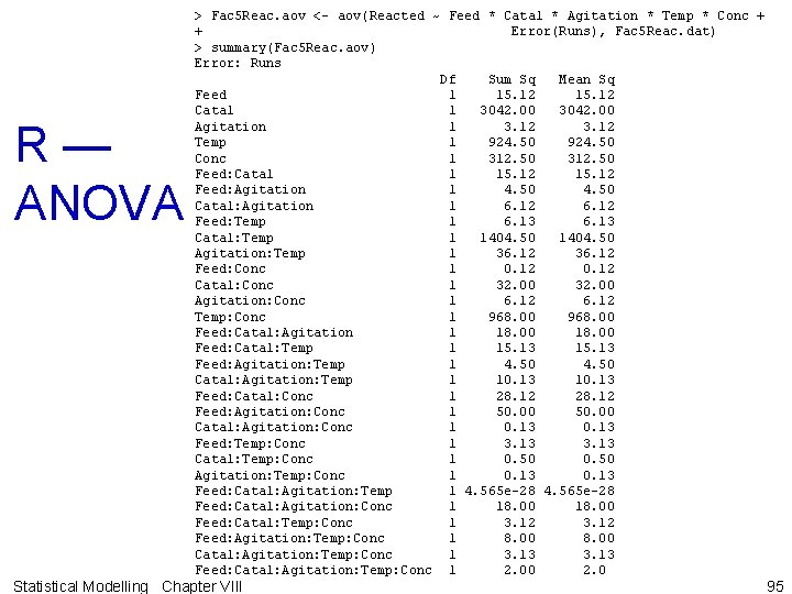
R — ANOVA > Fac 5 Reac. aov <- aov(Reacted ~ Feed * Catal * Agitation * Temp * Conc + + Error(Runs), Fac 5 Reac. dat) > summary(Fac 5 Reac. aov) Error: Runs Df Sum Sq Mean Sq Feed 1 15. 12 Catal 1 3042. 00 Agitation 1 3. 12 Temp 1 924. 50 Conc 1 312. 50 Feed: Catal 1 15. 12 Feed: Agitation 1 4. 50 Catal: Agitation 1 6. 12 Feed: Temp 1 6. 13 Catal: Temp 1 1404. 50 Agitation: Temp 1 36. 12 Feed: Conc 1 0. 12 Catal: Conc 1 32. 00 Agitation: Conc 1 6. 12 Temp: Conc 1 968. 00 Feed: Catal: Agitation 1 18. 00 Feed: Catal: Temp 1 15. 13 Feed: Agitation: Temp 1 4. 50 Catal: Agitation: Temp 1 10. 13 Feed: Catal: Conc 1 28. 12 Feed: Agitation: Conc 1 50. 00 Catal: Agitation: Conc 1 0. 13 Feed: Temp: Conc 1 3. 13 Catal: Temp: Conc 1 0. 50 Agitation: Temp: Conc 1 0. 13 Feed: Catal: Agitation: Temp 1 4. 565 e-28 Feed: Catal: Agitation: Conc 1 18. 00 Feed: Catal: Temp: Conc 1 3. 12 Feed: Agitation: Temp: Conc 1 8. 00 Catal: Agitation: Temp: Conc 1 3. 13 Feed: Catal: Agitation: Temp: Conc 1 2. 00 2. 0 Statistical Modelling Chapter VIII 95

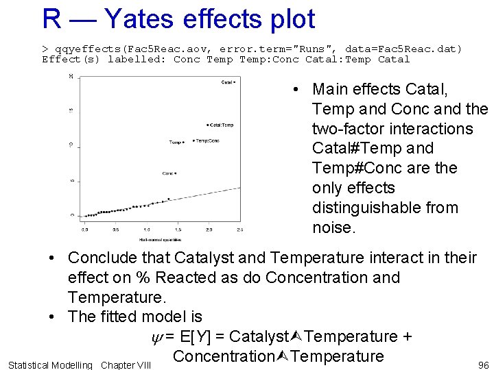
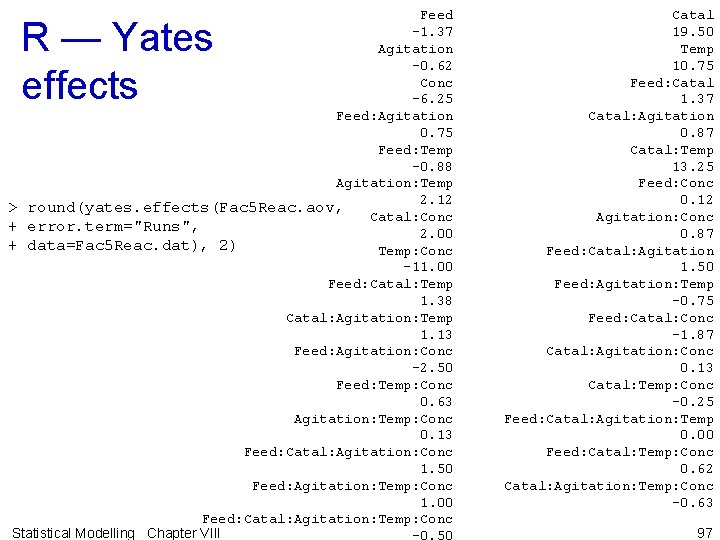
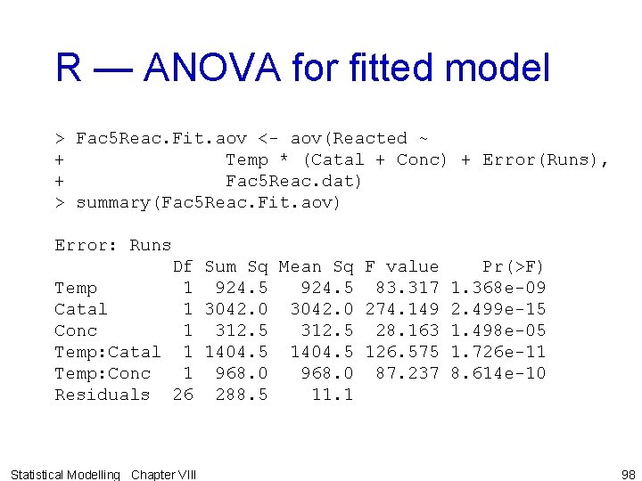
R — Yates effects plot > qqyeffects(Fac 5 Reac. aov, error. term="Runs", data=Fac 5 Reac. dat) Effect(s) labelled: Conc Temp: Conc Catal: Temp Catal • Main effects Catal, Temp and Conc and the two-factor interactions Catal#Temp and Temp#Conc are the only effects distinguishable from noise. • Conclude that Catalyst and Temperature interact in their effect on % Reacted as do Concentration and Temperature. • The fitted model is y = E[Y] = Catalyst Temperature + Concentration Temperature 96 Statistical Modelling Chapter VIII

Feed -1. 37 Agitation -0. 62 Conc -6. 25 Feed: Agitation 0. 75 Feed: Temp -0. 88 Agitation: Temp 2. 12 > round(yates. effects(Fac 5 Reac. aov, Catal: Conc + error. term="Runs", 2. 00 + data=Fac 5 Reac. dat), 2) Temp: Conc -11. 00 Feed: Catal: Temp 1. 38 Catal: Agitation: Temp 1. 13 Feed: Agitation: Conc -2. 50 Feed: Temp: Conc 0. 63 Agitation: Temp: Conc 0. 13 Feed: Catal: Agitation: Conc 1. 50 Feed: Agitation: Temp: Conc 1. 00 Feed: Catal: Agitation: Temp: Conc Statistical Modelling Chapter VIII R — Yates effects Catal 19. 50 Temp 10. 75 Feed: Catal 1. 37 Catal: Agitation 0. 87 Catal: Temp 13. 25 Feed: Conc 0. 12 Agitation: Conc 0. 87 Feed: Catal: Agitation 1. 50 Feed: Agitation: Temp -0. 75 Feed: Catal: Conc -1. 87 Catal: Agitation: Conc 0. 13 Catal: Temp: Conc -0. 25 Feed: Catal: Agitation: Temp 0. 00 Feed: Catal: Temp: Conc 0. 62 Catal: Agitation: Temp: Conc -0. 63 97

R — ANOVA for fitted model > Fac 5 Reac. Fit. aov <- aov(Reacted ~ + Temp * (Catal + Conc) + Error(Runs), + Fac 5 Reac. dat) > summary(Fac 5 Reac. Fit. aov) Error: Runs Df Sum Sq Mean Sq F value Pr(>F) Temp 1 924. 5 83. 317 1. 368 e-09 Catal 1 3042. 0 274. 149 2. 499 e-15 Conc 1 312. 5 28. 163 1. 498 e-05 Temp: Catal 1 1404. 5 126. 575 1. 726 e-11 Temp: Conc 1 968. 0 87. 237 8. 614 e-10 Residuals 26 288. 5 11. 1 Statistical Modelling Chapter VIII 98

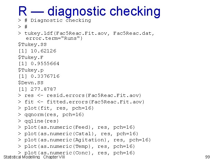
R — diagnostic checking > # Diagnostic checking > # > tukey. 1 df(Fac 5 Reac. Fit. aov, Fac 5 Reac. dat, error. term="Runs") $Tukey. SS [1] 10. 62126 $Tukey. F [1] 0. 9555664 $Tukey. p [1] 0. 3376716 $Devn. SS [1] 277. 8787 > res <- resid. errors(Fac 5 Reac. Fit. aov) > fit <- fitted. errors(Fac 5 Reac. Fit. aov) > plot(fit, res, pch=16) > qqnorm(res, pch=16) > qqline(res) > plot(as. numeric(Feed), res, pch=16) > plot(as. numeric(Catal), res, pch=16) > plot(as. numeric(Agitation), res, pch=16) > plot(as. numeric(Temp), res, pch=16) > plot(as. numeric(Conc), res, pch=16) Statistical Modelling Chapter VIII 99

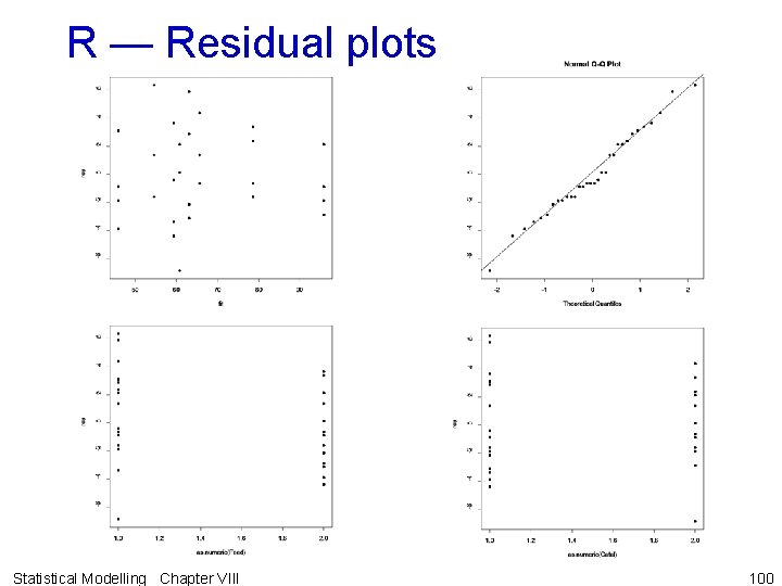
R — Residual plots Statistical Modelling Chapter VIII 100

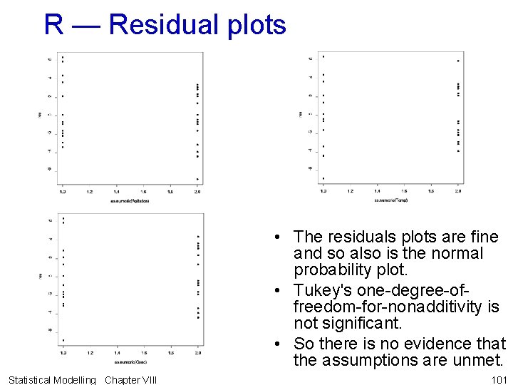
R — Residual plots • The residuals plots are fine and so also is the normal probability plot. • Tukey's one-degree-offreedom-for-nonadditivity is not significant. • So there is no evidence that the assumptions are unmet. Statistical Modelling Chapter VIII 101

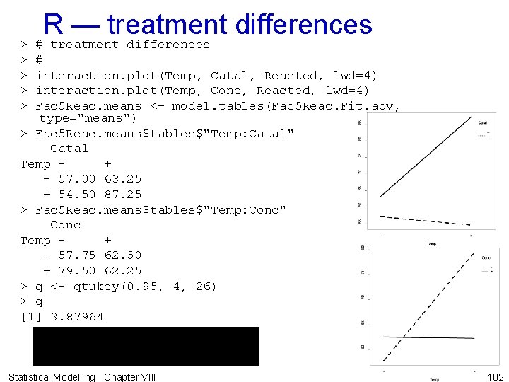
> > > R — treatment differences # interaction. plot(Temp, Catal, Reacted, lwd=4) interaction. plot(Temp, Conc, Reacted, lwd=4) Fac 5 Reac. means <- model. tables(Fac 5 Reac. Fit. aov, type="means") > Fac 5 Reac. means$tables$"Temp: Catal" Catal Temp + - 57. 00 63. 25 + 54. 50 87. 25 > Fac 5 Reac. means$tables$"Temp: Conc" Conc Temp + - 57. 75 62. 50 + 79. 50 62. 25 > q <- qtukey(0. 95, 4, 26) > q [1] 3. 87964 Statistical Modelling Chapter VIII 102

$a) Half-fractions of full factorial experiments • Definition VIII. 13: A 2 -pth fraction$

a) Half-fractions of full factorial experiments • Definition VIII. 13: A 2 -pth fraction of a 2 k experiment is designated a 2 k-p experiment. The number of runs in the experiment is equal to the value of 2 k-p. Construction of half-fractions • Rule VIII. 1: A 2 k-1 experiment is constructed as follows: – Write down a complete design in k-1 factors. – Compute the column of signs for factor k by forming the elementwise product of the columns of the complete design. That is, k = 123…(k-1). Statistical Modelling Chapter VIII 103

$Example VIII. 9 A halffraction of a 25 factorial experiment • Full factorial experiment$

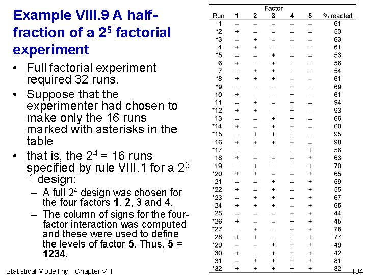
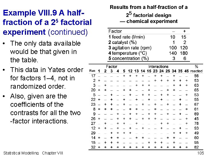
Example VIII. 9 A halffraction of a 25 factorial experiment • Full factorial experiment required 32 runs. • Suppose that the experimenter had chosen to make only the 16 runs marked with asterisks in the table • that is, the 24 = 16 runs specified by rule VIII. 1 for a 25 -1 design: – A full 24 design was chosen for the four factors 1, 2, 3 and 4. – The column of signs for the fourfactor interaction was computed and these were used to define the levels of factor 5. Thus, 5 = 1234. Statistical Modelling Chapter VIII 104

$Example VIII. 9 A halffraction of a 25 factorial experiment (continued) • The only$

Example VIII. 9 A halffraction of a 25 factorial experiment (continued) • The only data available would be that given in the table. • This data in Yates order for factors 1– 4, not in randomized order. • Also, given are the coefficients of the contrasts for all the two -factor interactions. Statistical Modelling Chapter VIII 105

$Aliasing in half-fractions • • • What has been lost in the half-fraction? Answer:$

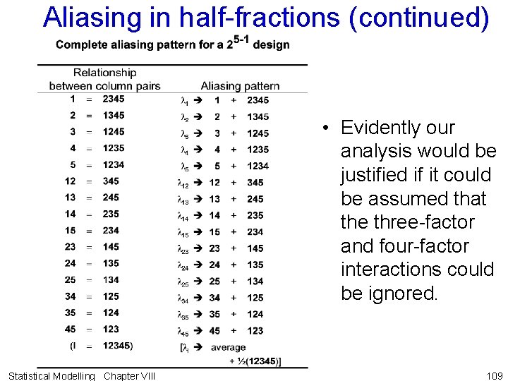
Aliasing in half-fractions • • • What has been lost in the half-fraction? Answer: various effects have been aliased. Definition VIII. 14: Two effects are said to be aliased when they are mixed up because of the deliberate use of only a fraction of the treatments. Compare this to confounding, where certain treatment effects are mixed up with block effects. Inability to separate effects arises from different actions: 1. because of the treatment combinations that the investigator chooses to observe; 2. because of the way treatments assigned to physical units. Statistical Modelling Chapter VIII 106

$Aliasing in half-fractions (continued) • In the table, only the columns for the main$

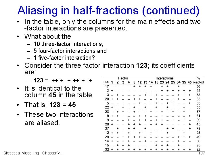
Aliasing in half-fractions (continued) • In the table, only the columns for the main effects and two -factor interactions are presented. • What about the – 10 three-factor interactions, – 5 four-factor interactions and – 1 five-factor interaction? • Consider the three factor interaction 123; its coefficients are: – 123 = -++-+--+ • It is identical to the column 45 in the table. • That is, 123 = 45 • These two interactions are aliased. Statistical Modelling Chapter VIII 107

$Aliasing in half-fractions (continued) • Now suppose we use 45 to denote the linear$

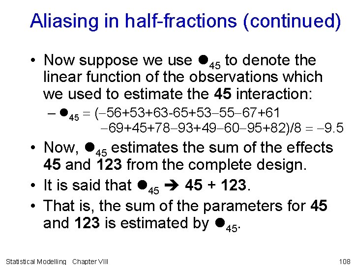
Aliasing in half-fractions (continued) • Now suppose we use 45 to denote the linear function of the observations which we used to estimate the 45 interaction: – 45 = (-56+53+63 -65+53 -55 -67+61 -69+45+78 -93+49 -60 -95+82)/8 = -9. 5 • Now, 45 estimates the sum of the effects 45 and 123 from the complete design. • It is said that 45 + 123. • That is, the sum of the parameters for 45 and 123 is estimated by 45. Statistical Modelling Chapter VIII 108

$Aliasing in half-fractions (continued) • Evidently our analysis would be justified if it could$

Aliasing in half-fractions (continued) • Evidently our analysis would be justified if it could be assumed that the three-factor and four-factor interactions could be ignored. Statistical Modelling Chapter VIII 109

$Analysis of half-fractions • The analysis of this set of 16 runs can still$

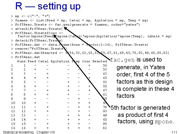
Analysis of half-fractions • The analysis of this set of 16 runs can still be accomplished using Yates algorithm since there are 4 factors for which it represents a full factorial. • However, R will perform the analysis producing lines for a set of unaliased terms. • The experimental structure is the same as for the full factorial. Statistical Modelling Chapter VIII 110

R — setting up > > > mp <- c("-", "+") fnames <- list(Feed = mp, Catal = mp, Agitation = mp, Temp = mp) Frf 5 Reac. Treats <- fac. gen(generate = fnames, order="yates") attach(Frf 5 Reac. Treats) Frf 5 Reac. Treats$Conc <factor(mpone(Feed)*mpone(Catal)*mpone(Agitation)*mpone(Temp), labels = mp) > detach(Frf 5 Reac. Treats) > Frf 5 Reac. dat <- data. frame(Runs = factor(1: 16), Frf 5 Reac. Treats) > remove("Frf 5 Reac. Treats") > Frf 5 Reac. dat$Reacted <- c(56, 53, 65, 53, 55, 67, 61, 69, 45, 78, 93, 49, 60, 95, 82) > Frf 5 Reac. dat Runs Feed Catal Agitation Temp Conc Reacted 1 1 + 56 2 2 + 53 3 3 + 63 4 4 + + + 65 5 5 + 53 6 6 + + + 55 7 7 + + + 67 8 8 + + + 61 9 9 + 69 10 10 + + + 45 11 11 + + + 78 12 12 + + + 93 13 13 + + + 49 14 14 + + + 60 15 15 + + + 95 16 16 + + + 82 111 Statistical Modelling Chapter VIII fac. gen is used to generate, in Yates order, first 4 of the 5 factors as this design is complete in these 4 factors 5 th factor is generated as product of first 4 factors, using mpone.

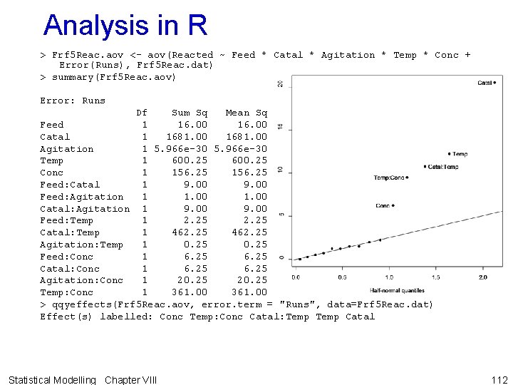
Analysis in R > Frf 5 Reac. aov <- aov(Reacted ~ Feed * Catal * Agitation * Temp * Conc + Error(Runs), Frf 5 Reac. dat) > summary(Frf 5 Reac. aov) Error: Runs Df Sum Sq Mean Sq Feed 1 16. 00 Catal 1 1681. 00 Agitation 1 5. 966 e-30 Temp 1 600. 25 Conc 1 156. 25 Feed: Catal 1 9. 00 Feed: Agitation 1 1. 00 Catal: Agitation 1 9. 00 Feed: Temp 1 2. 25 Catal: Temp 1 462. 25 Agitation: Temp 1 0. 25 Feed: Conc 1 6. 25 Catal: Conc 1 6. 25 Agitation: Conc 1 20. 25 Temp: Conc 1 361. 00 > qqyeffects(Frf 5 Reac. aov, error. term = "Runs", data=Frf 5 Reac. dat) Effect(s) labelled: Conc Temp: Conc Catal: Temp Catal Statistical Modelling Chapter VIII 112

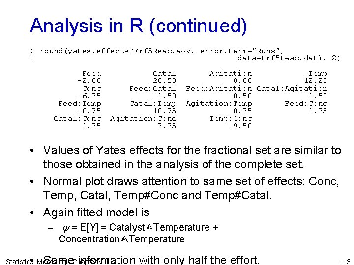
Analysis in R (continued) > round(yates. effects(Frf 5 Reac. aov, error. term="Runs", + data=Frf 5 Reac. dat), 2) Feed -2. 00 Conc -6. 25 Feed: Temp -0. 75 Catal: Conc 1. 25 Catal 20. 50 Feed: Catal 1. 50 Catal: Temp 10. 75 Agitation: Conc 2. 25 Agitation Temp 0. 00 12. 25 Feed: Agitation Catal: Agitation 0. 50 1. 50 Agitation: Temp Feed: Conc 0. 25 1. 25 Temp: Conc -9. 50 • Values of Yates effects for the fractional set are similar to those obtained in the analysis of the complete set. • Normal plot draws attention to same set of effects: Conc, Temp, Catal, Temp#Conc and Temp#Catal. • Again fitted model is – y = E[Y] = Catalyst Temperature + Concentration Temperature • Same information with only half the effort. Statistical Modelling Chapter VIII 113

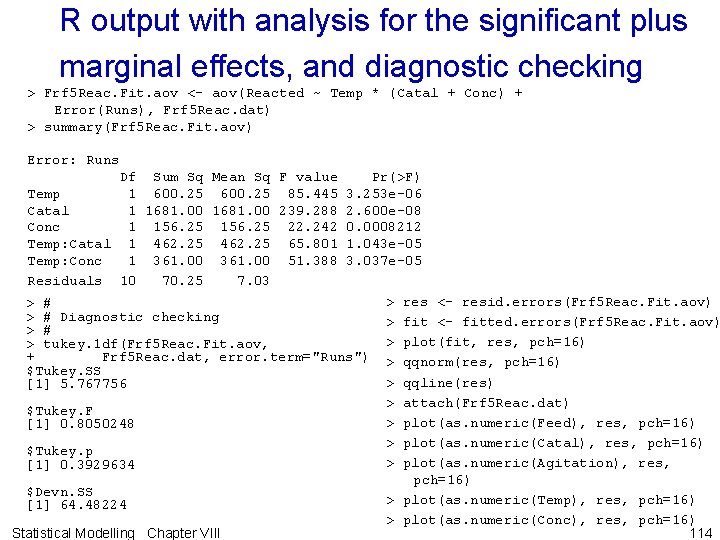
R output with analysis for the significant plus marginal effects, and diagnostic checking > Frf 5 Reac. Fit. aov <- aov(Reacted ~ Temp * (Catal + Conc) + Error(Runs), Frf 5 Reac. dat) > summary(Frf 5 Reac. Fit. aov) Error: Runs Df Sum Sq Mean Sq F value Pr(>F) Temp 1 600. 25 85. 445 3. 253 e-06 Catal 1 1681. 00 239. 288 2. 600 e-08 Conc 1 156. 25 22. 242 0. 0008212 Temp: Catal 1 462. 25 65. 801 1. 043 e-05 Temp: Conc 1 361. 00 51. 388 3. 037 e-05 Residuals 10 70. 25 7. 03 > res <- resid. errors(Frf 5 Reac. Fit. aov) > # Diagnostic checking > fit <- fitted. errors(Frf 5 Reac. Fit. aov) > # > plot(fit, res, pch=16) > tukey. 1 df(Frf 5 Reac. Fit. aov, + Frf 5 Reac. dat, error. term="Runs") > qqnorm(res, pch=16) $Tukey. SS > qqline(res) [1] 5. 767756 > attach(Frf 5 Reac. dat) $Tukey. F > plot(as. numeric(Feed), res, pch=16) [1] 0. 8050248 > plot(as. numeric(Catal), res, pch=16) $Tukey. p > plot(as. numeric(Agitation), res, [1] 0. 3929634 pch=16) $Devn. SS > plot(as. numeric(Temp), res, pch=16) [1] 64. 48224 > plot(as. numeric(Conc), res, pch=16) 114 Statistical Modelling Chapter VIII

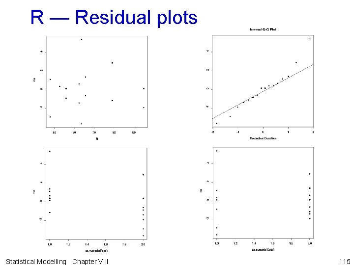
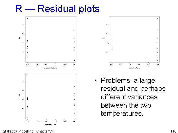
R — Residual plots Statistical Modelling Chapter VIII 115

R — Residual plots • Problems: a large residual and perhaps different variances between the two temperatures. Statistical Modelling Chapter VIII 116

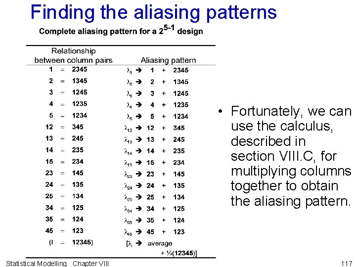
Finding the aliasing patterns • Fortunately, we can use the calculus, described in section VIII. C, for multiplying columns together to obtain the aliasing pattern. Statistical Modelling Chapter VIII 117

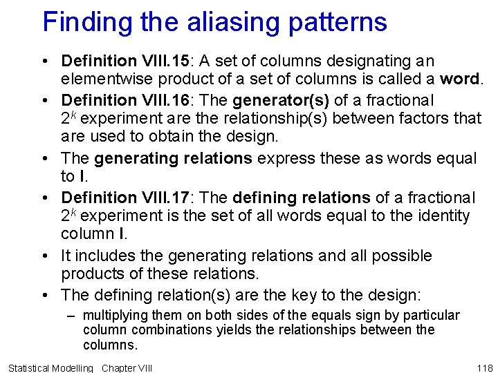
Finding the aliasing patterns • Definition VIII. 15: A set of columns designating an elementwise product of a set of columns is called a word. • Definition VIII. 16: The generator(s) of a fractional 2 k experiment are the relationship(s) between factors that are used to obtain the design. • The generating relations express these as words equal to I. • Definition VIII. 17: The defining relations of a fractional 2 k experiment is the set of all words equal to the identity column I. • It includes the generating relations and all possible products of these relations. • The defining relation(s) are the key to the design: – multiplying them on both sides of the equals sign by particular column combinations yields the relationships between the columns. Statistical Modelling Chapter VIII 118

$Example VIII. 9 A half-fraction of a 25 factorial experiment (continued) • The 25$

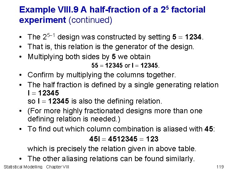
Example VIII. 9 A half-fraction of a 25 factorial experiment (continued) • The 25 -1 design was constructed by setting 5 = 1234. • That is, this relation is the generator of the design. • Multiplying both sides by 5 we obtain 55 = 12345 or I = 12345. • Confirm by multiplying the columns together. • The half fraction is defined by a single generating relation I = 12345 so I = 12345 is also the defining relation. • (For more highly fractionated designs more than one defining relation is needed. ) • To find out which column combination is aliased with 45: 45 I = 4512345 = 123 which is precisely the relation given in above table. • The other aliasing relations can be found similarly. Statistical Modelling Chapter VIII 119

$b) More on construction and use of half-factions • The complimentary half-fraction • Definition$

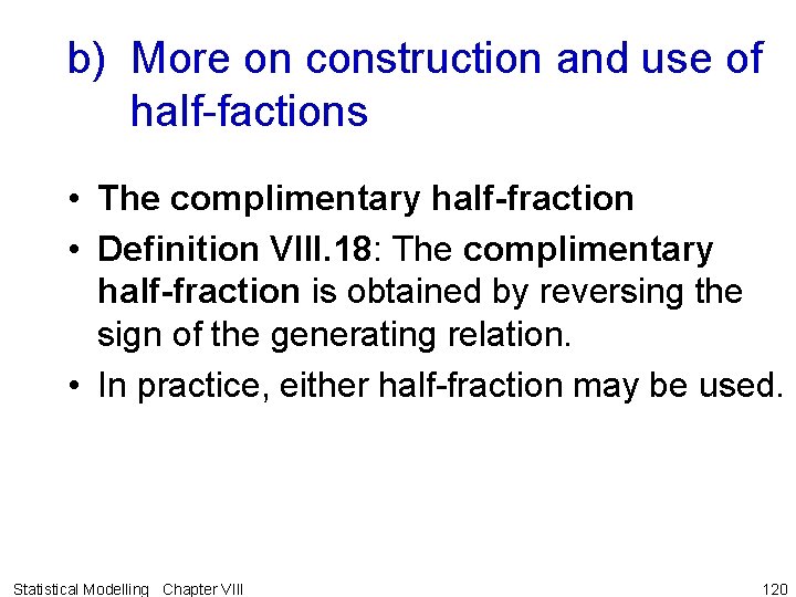
b) More on construction and use of half-factions • The complimentary half-fraction • Definition VIII. 18: The complimentary half-fraction is obtained by reversing the sign of the generating relation. • In practice, either half-fraction may be used. Statistical Modelling Chapter VIII 120

$Example VIII. 9 A half-fraction of a 25 factorial experiment (continued) • Design was$

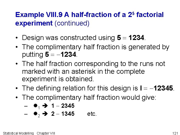
Example VIII. 9 A half-fraction of a 25 factorial experiment (continued) • Design was constructed using 5 = 1234. • The complimentary half fraction is generated by putting 5 = -1234. • The half fraction corresponding to the runs not marked with an asterisk in the complete experiment is obtained. • The defining relation for this design is I = -12345. • The complimentary half fraction would give: – 1 1 - 2345 – 2 2 - 1345 Statistical Modelling Chapter VIII etc. 121

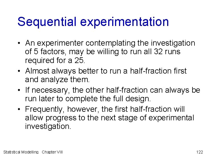
Sequential experimentation • An experimenter contemplating the investigation of 5 factors, may be willing to run all 32 runs required for a 25. • Almost always better to run a half-fraction first and analyze them. • If necessary, the other half-fraction can always be run later to complete the full design. • Frequently, however, the first half-fraction will allow progress to the next stage of experimental investigation. Statistical Modelling Chapter VIII 122

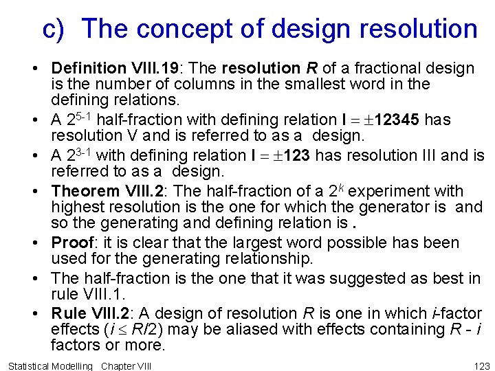
c) The concept of design resolution • Definition VIII. 19: The resolution R of a fractional design is the number of columns in the smallest word in the defining relations. • A 25 -1 half-fraction with defining relation I = 12345 has resolution V and is referred to as a design. • A 23 -1 with defining relation I = 123 has resolution III and is referred to as a design. • Theorem VIII. 2: The half-fraction of a 2 k experiment with highest resolution is the one for which the generator is and so the generating and defining relation is. • Proof: it is clear that the largest word possible has been used for the generating relationship. • The half-fraction is the one that it was suggested as best in rule VIII. 1. • Rule VIII. 2: A design of resolution R is one in which i-factor effects (i R/2) may be aliased with effects containing R - i factors or more. Statistical Modelling Chapter VIII 123

$Example VIII. 9 A half-fraction of a 25 factorial experiment (continued) • The 25$

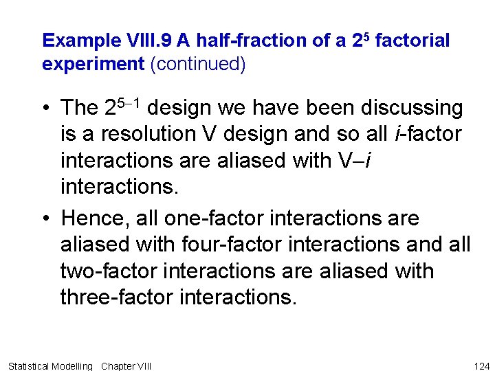
Example VIII. 9 A half-fraction of a 25 factorial experiment (continued) • The 25 -1 design we have been discussing is a resolution V design and so all i-factor interactions are aliased with V-i interactions. • Hence, all one-factor interactions are aliased with four-factor interactions and all two-factor interactions are aliased with three-factor interactions. Statistical Modelling Chapter VIII 124

$c) The concept of design resolution (continued) • For the various sized fractions of$

c) The concept of design resolution (continued) • For the various sized fractions of a 2 k: 1. a design of resolution III does not alias main effects with one another, but does alias main effects with two factor interactions; 2. a design of resolution IV does not alias main effects and two-factor interactions, but does alias two factor interactions with one another; 3. a design of resolution V does not alias main effects and two-factor with one another, but does alias two factor interactions with threefactor interactions. Statistical Modelling Chapter VIII 125

Embedded factorials • One of the very important aspects of resolution is that a fractional factorial design of resolution R contains complete factorials (possibly replicated) in every set of R-1 factors. • Suppose then that an experimenter has a number of candidate factors but believes that all but R-1 of them (specific identity unknown) may have no detectable effects. • If she employs a fractional factorial design of resolution R she will have a complete factorial design in the effective factors. Statistical Modelling Chapter VIII 126

$Example VIII. 9 A half-fraction of a 25 factorial experiment (continued) • The design$

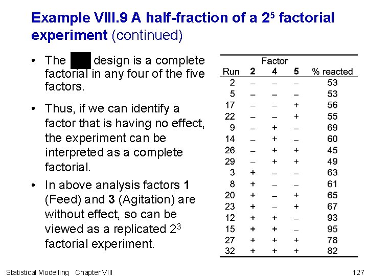
Example VIII. 9 A half-fraction of a 25 factorial experiment (continued) • The design is a complete factorial in any four of the five factors. • Thus, if we can identify a factor that is having no effect, the experiment can be interpreted as a complete factorial. • In above analysis factors 1 (Feed) and 3 (Agitation) are without effect, so can be viewed as a replicated 23 factorial experiment. Statistical Modelling Chapter VIII 127

d) Resolution III designs (also called main effect plans) • In a resolution III design, the main effects are aliased with two-factor interactions. • Can construct resolution III designs for up to k = n-1 factors, where n is a multiple of 4. • Particularly important subset are those for which n is a power of 2. In particular, – up to 3 factors in 4 runs, – up to 7 factors in 8 runs and – up to 15 factors in 16 runs. • Definition VIII. 20: A fractional design is said to be a saturated design if the number of factors k = n-1; that is, all contrasts are associated with main effects. • Saturated designs at heart of Taguchi quality control methods which have been attributed as being the basis of Japanese industrial supremacy. – They used these designs in developing products to determine which factors affect product quality. • In using these designs assuming all two-factor interactions are negligible. • Not so useful in agriculture. Statistical Modelling Chapter VIII 128

Resolution III designs for which n is a power of 2 • Rule VIII. 3: designs in which n = 2 k-p are constructed as follows: 1. Write down a complete design in k-p factors. 2. Compute the column of signs for additional factors by associating the factors with the interaction columns of the factors in the complete design. • We will now investigate the use of resolution III designs. Statistical Modelling Chapter VIII 129

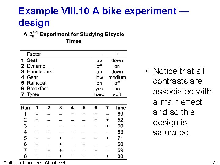
Example VIII. 10 A bike experiment • Consider the following experiment designed to investigate the effects of 7 factors on the time it takes a particular person to cycle up a hill. • That is, it is a one sixteenth fraction of a 27 experiment involving 23 = 8 runs. • The design is constructed by: 1. writing down a full factorial design for the three variables 1, 2 and 3; 2. the additional variables 4, 5, 6 and 7 are associated with all the interaction columns 12, 13, 23 and 123, respectively. • Hence, the generating relations of the design are I = 124, I = 135, I = 236, I = 1237. Statistical Modelling Chapter VIII 130

Example VIII. 10 A bike experiment — design • Notice that all contrasts are associated with a main effect and so this design is saturated. Statistical Modelling Chapter VIII 131

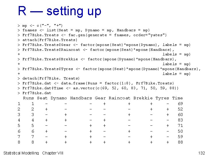
R — setting up > > > + > + > > mp <- c("-", "+") fnames <- list(Seat = mp, Dynamo = mp, Handbars = mp) Frf 7 Bike. Treats <- fac. gen(generate = fnames, order="yates") attach(Frf 7 Bike. Treats) Frf 7 Bike. Treats$Gear <- factor(mpone(Seat)*mpone(Dynamo), labels = mp) Frf 7 Bike. Treats$Raincoat <- factor(mpone(Seat)*mpone(Handbars), labels = mp) Frf 7 Bike. Treats$Brekkie <- factor(mpone(Dynamo)*mpone(Handbars), labels = mp) Frf 7 Bike. Treats$Tyres <- factor(mpone(Seat)*mpone(Dynamo)*mpone(Handbars), labels = mp) detach(Frf 7 Bike. Treats) Frf 7 Bike. dat <- data. frame(Runs = factor(1: 8), Frf 7 Bike. Treats) Frf 7 Bike. dat$Time <- as. vector(c(69, 52, 60, 83, 71, 50, 59, 88)) Frf 7 Bike. dat 1 2 3 4 5 6 7 8 Runs Seat Dynamo Handbars Gear Raincoat Brekkie Tyres Time 1 + + + 69 2 + + + 52 3 + + + 60 4 + + + 83 5 + + + 71 6 + + + 50 7 + + + 59 8 + + + + 88 Statistical Modelling Chapter VIII 132

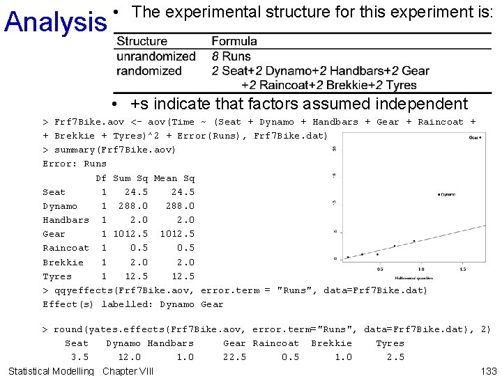
Analysis • The experimental structure for this experiment is: • +s indicate that factors assumed independent > Frf 7 Bike. aov <- aov(Time ~ (Seat + Dynamo + Handbars + Gear + Raincoat + + Brekkie + Tyres)^2 + Error(Runs), Frf 7 Bike. dat) > summary(Frf 7 Bike. aov) Error: Runs Df Sum Sq Mean Sq Seat 1 24. 5 Dynamo 1 288. 0 Handbars 1 2. 0 Gear 1 1012. 5 Raincoat 1 0. 5 Brekkie 1 2. 0 Tyres 1 12. 5 > qqyeffects(Frf 7 Bike. aov, error. term = "Runs", data=Frf 7 Bike. dat) Effect(s) labelled: Dynamo Gear > round(yates. effects(Frf 7 Bike. aov, error. term="Runs", data=Frf 7 Bike. dat), 2) Seat Dynamo Handbars Gear Raincoat Brekkie Tyres 3. 5 12. 0 1. 0 22. 5 0. 5 1. 0 2. 5 133 Statistical Modelling Chapter VIII

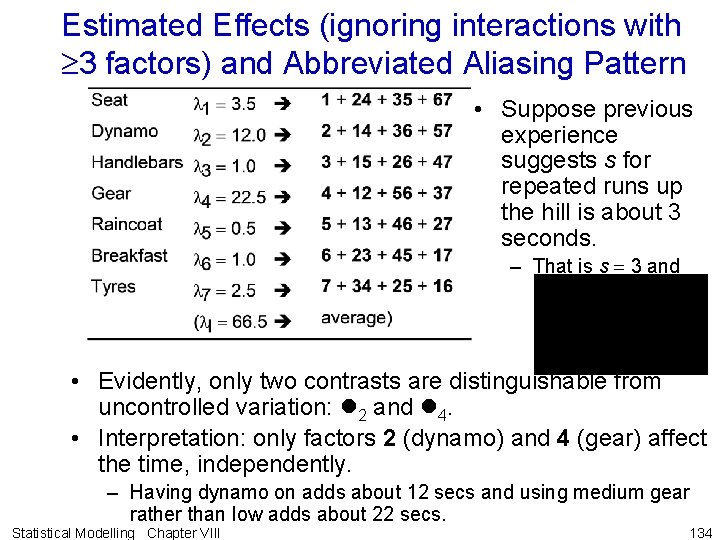
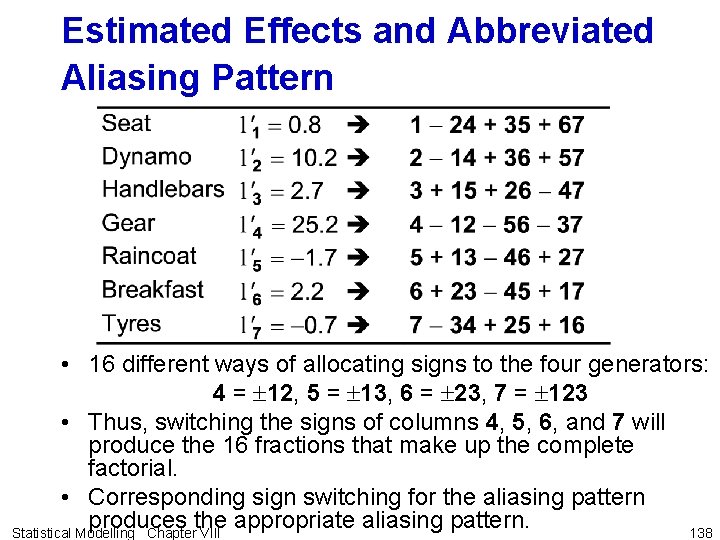
Estimated Effects (ignoring interactions with 3 factors) and Abbreviated Aliasing Pattern • Suppose previous experience suggests s for repeated runs up the hill is about 3 seconds. – That is s = 3 and • Evidently, only two contrasts are distinguishable from uncontrolled variation: 2 and 4. • Interpretation: only factors 2 (dynamo) and 4 (gear) affect the time, independently. – Having dynamo on adds about 12 secs and using medium gear rather than low adds about 22 secs. Statistical Modelling Chapter VIII 134

Problem • However, there is some ambiguity in these conclusions. • May be, for example, that 4 is large, not because of a large main effect 4, but because one or more of the interactions 12, 56 and 37 are large. • A further experiment would concentrate on factor 4 to confirm that there is a large main effect for this factor. • Also, note that, being a resolution III design, it will contain complete 22 factorial experiments replicated twice in every pair of factors. • Thus, it contains a complete factorial in factors 2 and 4. Statistical Modelling Chapter VIII 135

$Other fractions • The design we have used is only one particular 1/16 fraction$

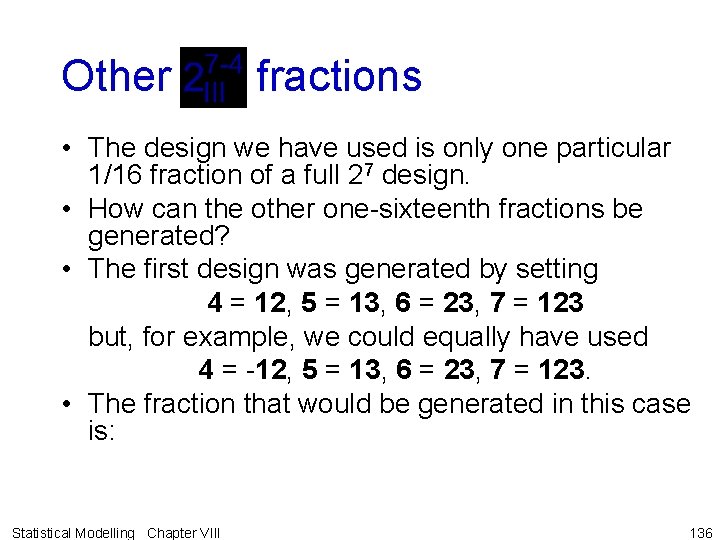
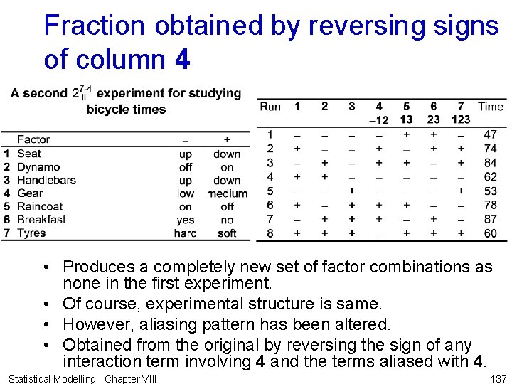
Other fractions • The design we have used is only one particular 1/16 fraction of a full 27 design. • How can the other one-sixteenth fractions be generated? • The first design was generated by setting 4 = 12, 5 = 13, 6 = 23, 7 = 123 but, for example, we could equally have used 4 = -12, 5 = 13, 6 = 23, 7 = 123. • The fraction that would be generated in this case is: Statistical Modelling Chapter VIII 136

Fraction obtained by reversing signs of column 4 • Produces a completely new set of factor combinations as none in the first experiment. • Of course, experimental structure is same. • However, aliasing pattern has been altered. • Obtained from the original by reversing the sign of any interaction term involving 4 and the terms aliased with 4. Statistical Modelling Chapter VIII 137

Estimated Effects and Abbreviated Aliasing Pattern • 16 different ways of allocating signs to the four generators: 4 = 12, 5 = 13, 6 = 23, 7 = 123 • Thus, switching the signs of columns 4, 5, 6, and 7 will produce the 16 fractions that make up the complete factorial. • Corresponding sign switching for the aliasing pattern produces the appropriate aliasing pattern. 138 Statistical Modelling Chapter VIII

$Combining two fractions • Suppose that the results of the two fractional experiments were$

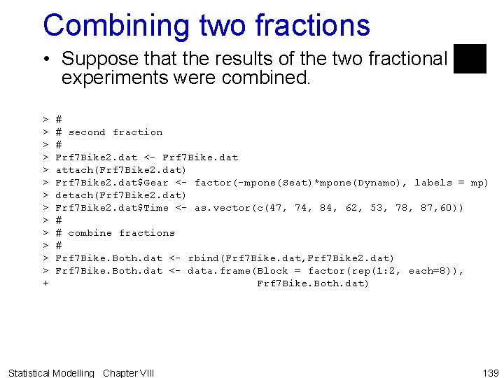
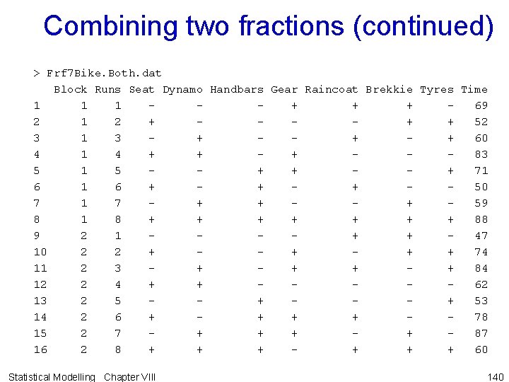
Combining two fractions • Suppose that the results of the two fractional experiments were combined. > > > > + # # second fraction # Frf 7 Bike 2. dat <- Frf 7 Bike. dat attach(Frf 7 Bike 2. dat) Frf 7 Bike 2. dat$Gear <- factor(-mpone(Seat)*mpone(Dynamo), labels = mp) detach(Frf 7 Bike 2. dat) Frf 7 Bike 2. dat$Time <- as. vector(c(47, 74, 84, 62, 53, 78, 87, 60)) # # combine fractions # Frf 7 Bike. Both. dat <- rbind(Frf 7 Bike. dat, Frf 7 Bike 2. dat) Frf 7 Bike. Both. dat <- data. frame(Block = factor(rep(1: 2, each=8)), Frf 7 Bike. Both. dat) Statistical Modelling Chapter VIII 139

$Combining two fractions (continued) > Frf 7 Bike. Both. dat Block Runs Seat Dynamo$

Combining two fractions (continued) > Frf 7 Bike. Both. dat Block Runs Seat Dynamo Handbars Gear Raincoat Brekkie Tyres Time 1 1 1 + + + 69 2 1 2 + + + 52 3 1 3 + + + 60 4 1 4 + + + 83 5 1 5 + + + 71 6 + + + 50 7 1 7 + + + 59 8 1 8 + + + + 88 9 2 1 + + 47 10 2 2 + + 74 11 2 3 + + 84 12 2 4 + + 62 13 2 5 + + 53 14 2 6 + + 78 15 2 7 + + 87 16 2 8 + + + 60 Statistical Modelling Chapter VIII 140

$Combining two fractions (continued) • As it will now be possible to estimate interactions,$

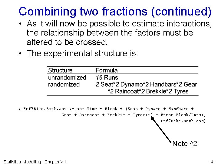
Combining two fractions (continued) • As it will now be possible to estimate interactions, the relationship between the factors must be altered to be crossed. • The experimental structure is: > Frf 7 Bike. Both. aov <- aov(Time ~ Block + (Seat + Dynamo + Handbars + Gear + Raincoat + Brekkie + Tyres)^2 + Error(Block/Runs), Frf 7 Bike. Both. dat) Note ^2 Statistical Modelling Chapter VIII 141

$Combining two fractions (continued) > summary(Frf 7 Bike. Both. aov) Error: Block Df Sum$

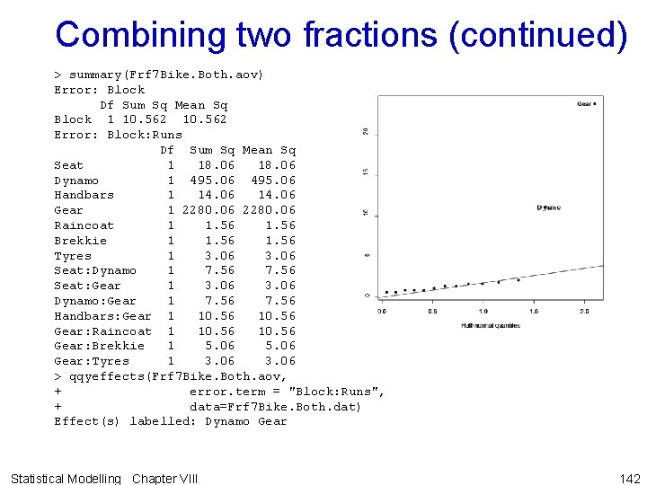
Combining two fractions (continued) > summary(Frf 7 Bike. Both. aov) Error: Block Df Sum Sq Mean Sq Block 1 10. 562 Error: Block: Runs Df Sum Sq Mean Sq Seat 1 18. 06 Dynamo 1 495. 06 Handbars 1 14. 06 Gear 1 2280. 06 Raincoat 1 1. 56 Brekkie 1 1. 56 Tyres 1 3. 06 Seat: Dynamo 1 7. 56 Seat: Gear 1 3. 06 Dynamo: Gear 1 7. 56 Handbars: Gear 1 10. 56 Gear: Raincoat 1 10. 56 Gear: Brekkie 1 5. 06 Gear: Tyres 1 3. 06 > qqyeffects(Frf 7 Bike. Both. aov, + error. term = "Block: Runs", + data=Frf 7 Bike. Both. dat) Effect(s) labelled: Dynamo Gear Statistical Modelling Chapter VIII 142

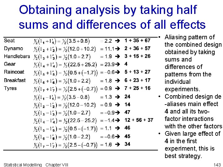
Obtaining analysis by taking half sums and differences of all effects • Aliasing pattern of the combined design obtained by taking sums and differences of patterns from the individual experiments. • Combined design de -aliases main effect 4 and all its twofactor interactions with the other factors. • Given large effect of 4 in the first experiment, this is best strategy. Statistical Modelling Chapter VIII 143

$Utility of sequential fractionals • Thus, the use of fractional factorials sequentially is a$

Utility of sequential fractionals • Thus, the use of fractional factorials sequentially is a very useful application of them. • Also possible to add fraction to original to de-alias all main effects, leaving 2 -factor interactions aliased in groups of 3. Statistical Modelling Chapter VIII 144

Plackett and Burman Designs • Definition VIII. 21: Plackett and Burman designs are two-level fractional factorial designs for studying k = n-1 factors in n runs where n is a multiple of 4. • n a power of 2 identical to those already presented. • Designs for n = 12, 20, 24, 28 and 30 are sometimes of interest. Statistical Modelling Chapter VIII 145

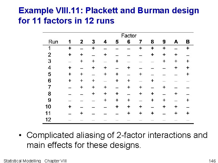
Example VIII. 11: Plackett and Burman design for 11 factors in 12 runs • Complicated aliasing of 2 -factor interactions and main effects for these designs. Statistical Modelling Chapter VIII 146

$e) Table of fractional factorial designs • The following table is an extract from$

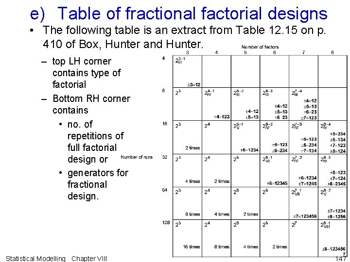
e) Table of fractional factorial designs • The following table is an extract from Table 12. 15 on p. 410 of Box, Hunter and Hunter. – top LH corner contains type of factorial – Bottom RH corner contains • no. of repetitions of full factorial design or • generators for fractional design. Statistical Modelling Chapter VIII 147

$e) Table of fractional factorial designs (continued) – To use this table, examine •$

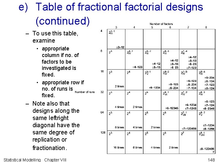
e) Table of fractional factorial designs (continued) – To use this table, examine • appropriate column if no. of factors to be investigated is fixed. • appropriate row if no. of runs is fixed. – Note also that designs along the same leftright diagonal have the same degree of replication or fractionation. Statistical Modelling Chapter VIII 148