ANOVA FACTORIAL DESIGN Factorial design Factorial design an

ANOVA: FACTORIAL DESIGN

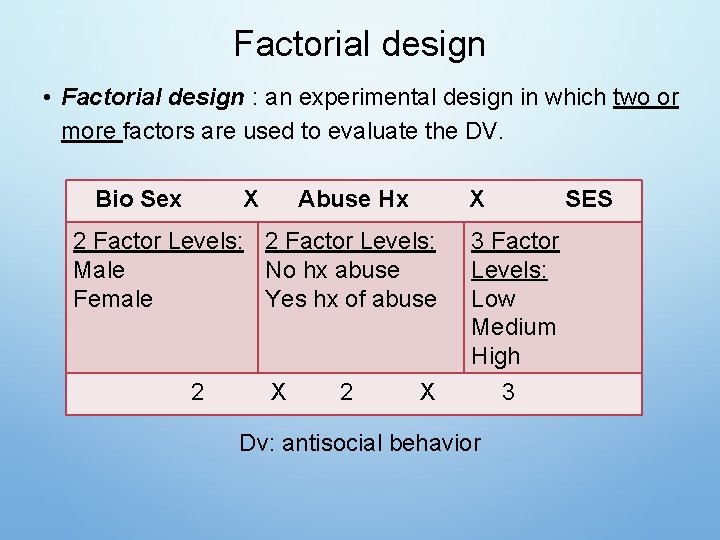
Factorial design • Factorial design : an experimental design in which two or more factors are used to evaluate the DV. Bio Sex X Abuse Hx X 2 Factor Levels: Male No hx abuse Female Yes hx of abuse 2 X 3 Factor Levels: Low Medium High 3 Dv: antisocial behavior SES

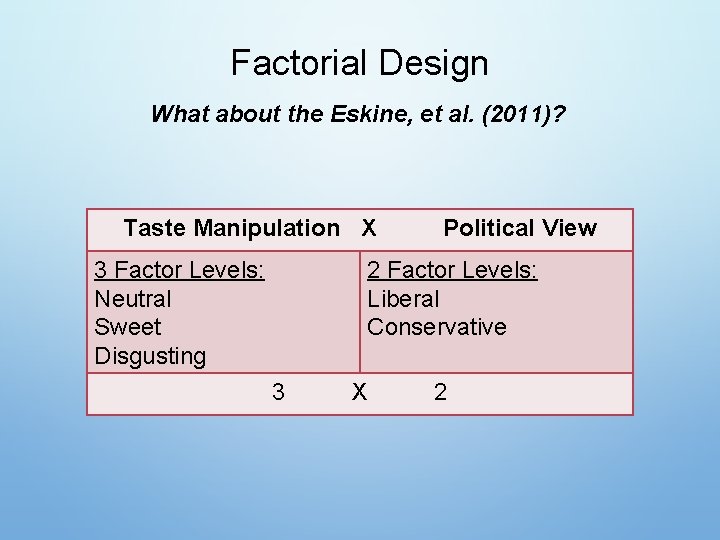
Factorial Design What about the Eskine, et al. (2011)? Taste Manipulation X 3 Factor Levels: Neutral Sweet Disgusting Political View 2 Factor Levels: Liberal Conservative 3 X 2

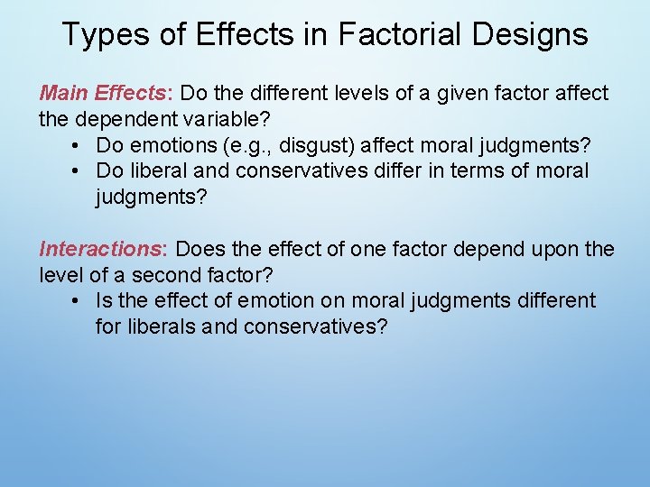
Types of Effects in Factorial Designs Main Effects: Do the different levels of a given factor affect the dependent variable? • Do emotions (e. g. , disgust) affect moral judgments? • Do liberal and conservatives differ in terms of moral judgments? Interactions: Does the effect of one factor depend upon the level of a second factor? • Is the effect of emotion on moral judgments different for liberals and conservatives?

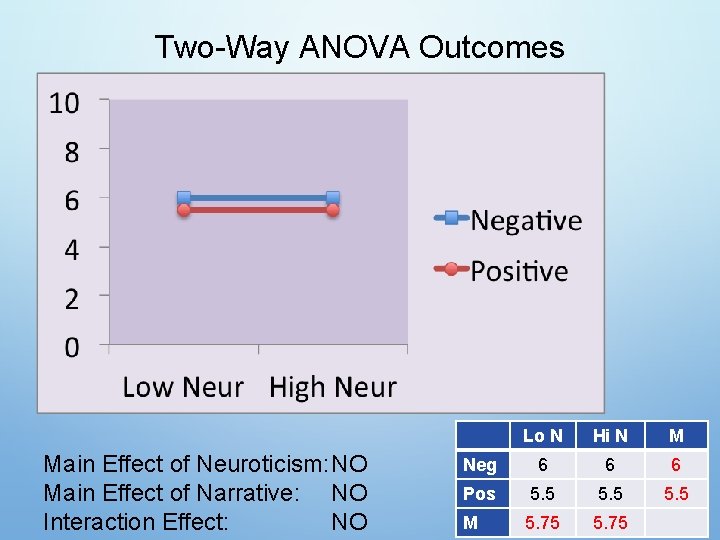
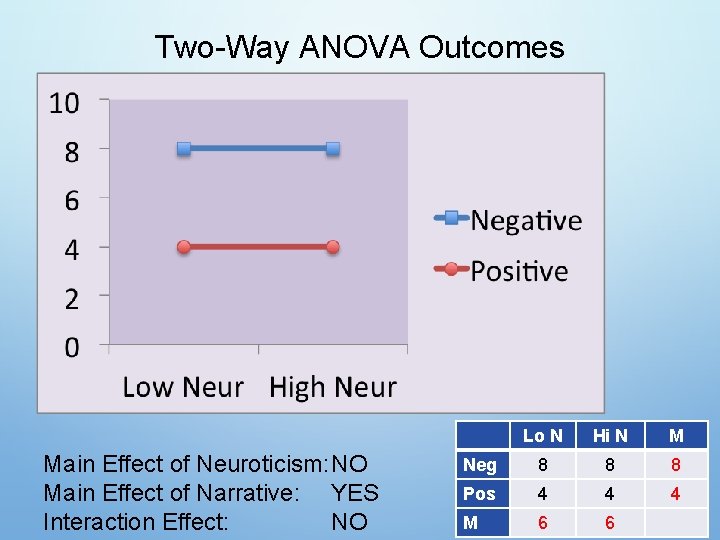
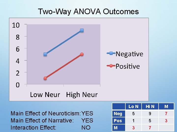
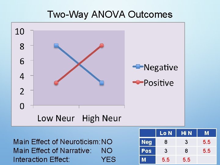
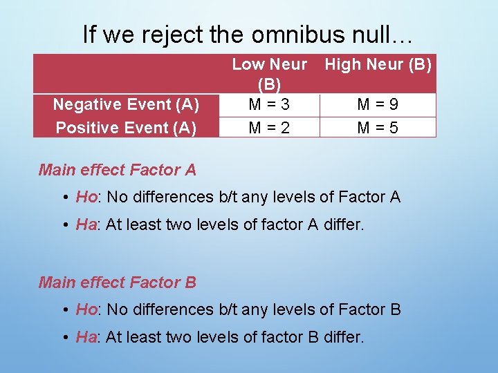
Two-way ANOVA Research suggests that personality is reflected in the way people talk and write about past experiences. An experiment was conducted in which individuals who were either high or low in neuroticism wrote a narrative about either a positive or a negative experience from their past. The research question was whether neuroticism would predict the number of negative emotion words included in the narrative in each narrative and whether the pattern of negativity would vary as a function of the narrative type.

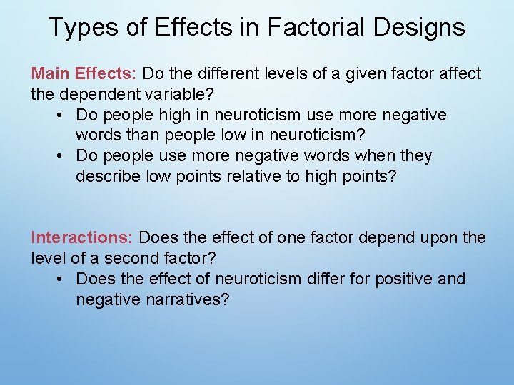
Types of Effects in Factorial Designs Main Effects: Do the different levels of a given factor affect the dependent variable? • Do people high in neuroticism use more negative words than people low in neuroticism? • Do people use more negative words when they describe low points relative to high points? Interactions: Does the effect of one factor depend upon the level of a second factor? • Does the effect of neuroticism differ for positive and negative narratives?

Two-Way ANOVA Outcomes Main Effect of Neuroticism: NO Main Effect of Narrative: NO Interaction Effect: NO Lo N Hi N M Neg 6 6 6 Pos 5. 5 M 5. 75

Two-Way ANOVA Outcomes Main Effect of Neuroticism: YES Main Effect of Narrative: NO Interaction Effect: NO Lo N Hi N M Neg 3 9 6 Pos 2. 5 8. 5 5. 5 M 2. 75 8. 75

Two-Way ANOVA Outcomes Main Effect of Neuroticism: NO Main Effect of Narrative: YES Interaction Effect: NO Lo N Hi N M Neg 8 8 8 Pos 4 4 4 M 6 6

Two-Way ANOVA Outcomes Main Effect of Neuroticism: YES Main Effect of Narrative: YES Interaction Effect: NO Lo N Hi N M Neg 5 9 7 Pos 1 5 3 M 3 7

Two-Way ANOVA Outcomes Main Effect of Neuroticism: YES Main Effect of Narrative: YES Interaction Effect: YES Lo N Hi N M Neg 3 9 6 Pos 2 5 3. 5 2. 5 7 M

Two-Way ANOVA Outcomes Main Effect of Neuroticism: NO Main Effect of Narrative: NO Interaction Effect: YES Lo N Hi N M Neg 8 3 5. 5 Pos 3 8 5. 5 M

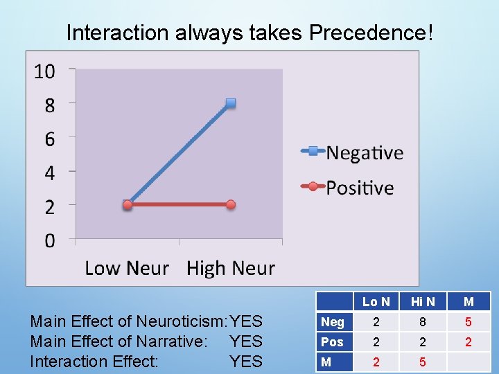
Interaction always takes Precedence! Main Effect of Neuroticism: YES Main Effect of Narrative: YES Interaction Effect: YES Lo N Hi N M Neg 2 8 5 Pos 2 2 2 M 2 5

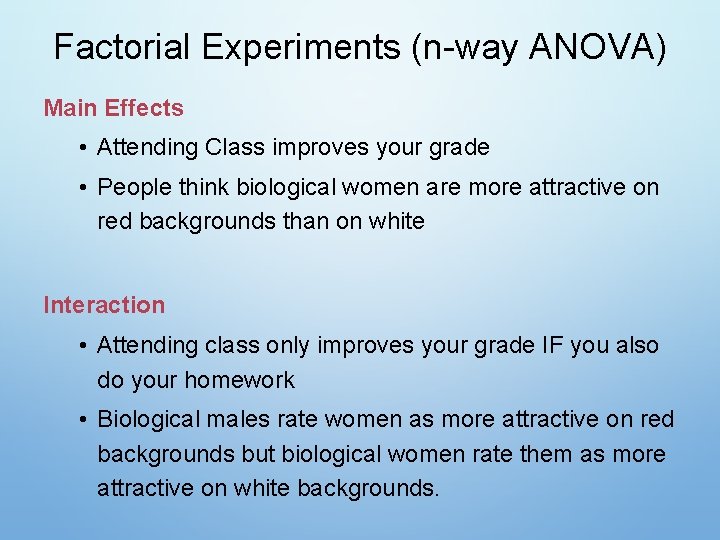
Factorial Experiments (n-way ANOVA) Main Effects • Attending Class improves your grade • People think biological women are more attractive on red backgrounds than on white Interaction • Attending class only improves your grade IF you also do your homework • Biological males rate women as more attractive on red backgrounds but biological women rate them as more attractive on white backgrounds.

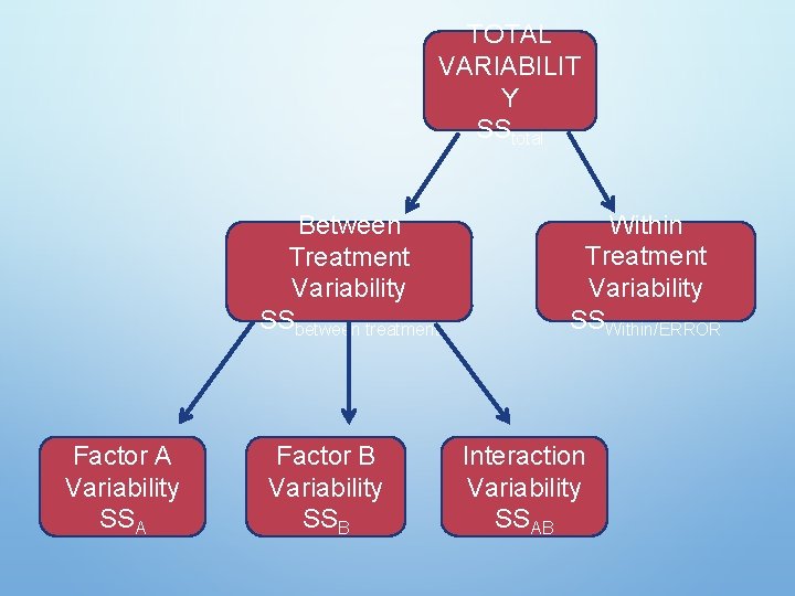
TOTAL VARIABILIT Y SStotal Between Treatment Variability SSbetween treatment Factor A Variability SSA Factor B Variability SSB Within Treatment Variability SSWithin/ERROR Interaction Variability SSAB

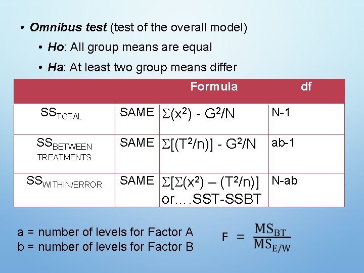
• Omnibus test (test of the overall model) • Ho: All group means are equal • Ha: At least two group means differ Formula SSTOTAL SSBETWEEN df SAME (x 2) - G 2/N N-1 SAME [(T 2/n)] - G 2/N ab-1 SAME [ (x 2) – (T 2/n)] N-ab TREATMENTS SSWITHIN/ERROR or…. SST-SSBT a = number of levels for Factor A b = number of levels for Factor B

If we reject the omnibus null… Negative Event (A) Positive Event (A) Low Neur (B) M=3 M=2 High Neur (B) M=9 M=5 Main effect Factor A • Ho: No differences b/t any levels of Factor A • Ha: At least two levels of factor A differ. Main effect Factor B • Ho: No differences b/t any levels of Factor B • Ha: At least two levels of factor B differ.

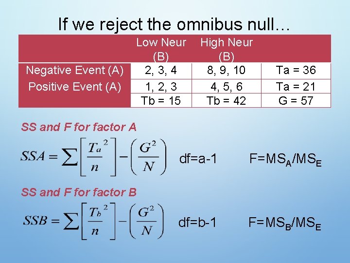
If we reject the omnibus null… Negative Event (A) Positive Event (A) Low Neur (B) 2, 3, 4 1, 2, 3 Tb = 15 High Neur (B) 8, 9, 10 4, 5, 6 Tb = 42 Ta = 36 Ta = 21 G = 57 SS and F for factor A df=a-1 F=MSA/MSE df=b-1 F=MSB/MSE SS and F for factor B

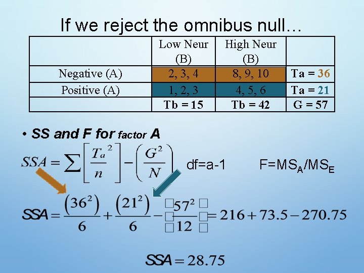
If we reject the omnibus null… Negative (A) Positive (A) Low Neur (B) 2, 3, 4 1, 2, 3 Tb = 15 High Neur (B) 8, 9, 10 4, 5, 6 Tb = 42 Ta = 36 Ta = 21 G = 57 • SS and F for factor A df=a-1 F=MSA/MSE

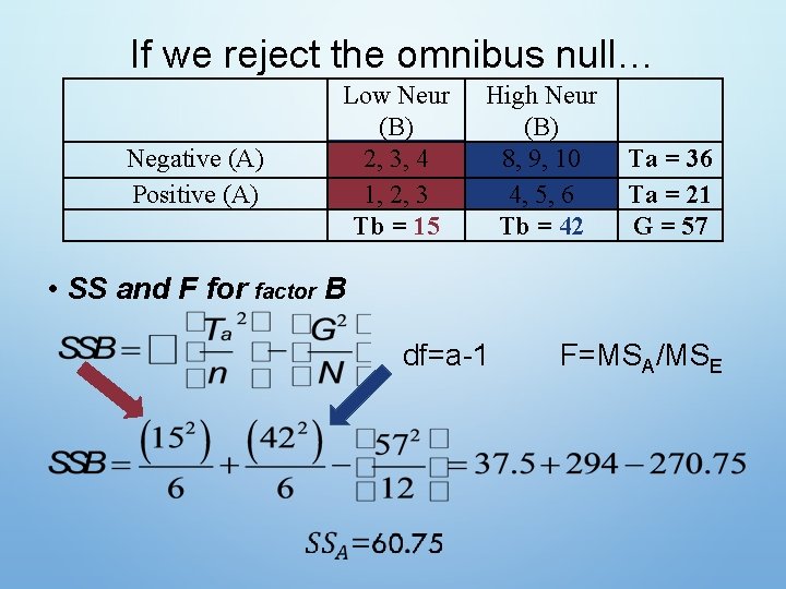
If we reject the omnibus null… Negative (A) Positive (A) Low Neur (B) 2, 3, 4 1, 2, 3 Tb = 15 High Neur (B) 8, 9, 10 4, 5, 6 Tb = 42 Ta = 36 Ta = 21 G = 57 • SS and F for factor B df=a-1 F=MSA/MSE

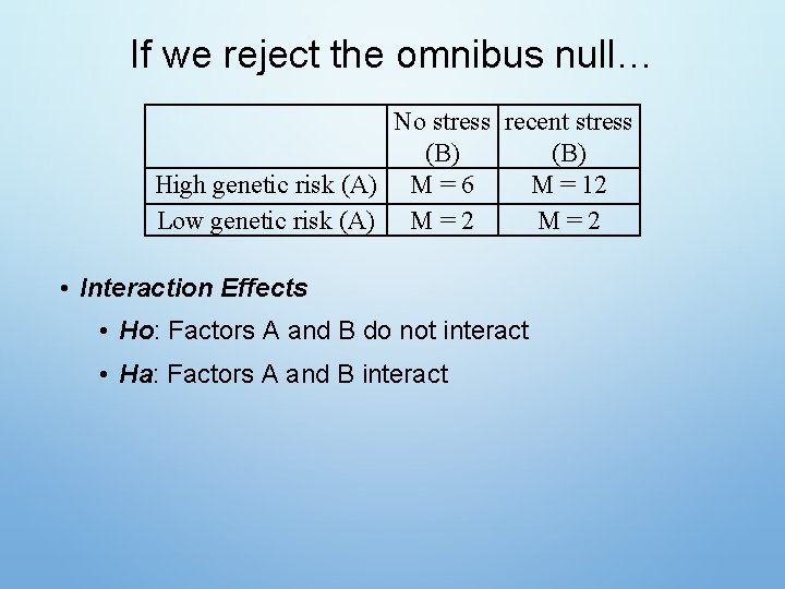
If we reject the omnibus null… No stress recent stress (B) High genetic risk (A) M = 6 M = 12 Low genetic risk (A) M = 2 M=2 • Interaction Effects • Ho: Factors A and B do not interact • Ha: Factors A and B interact

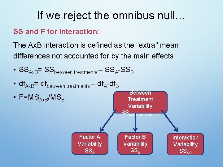
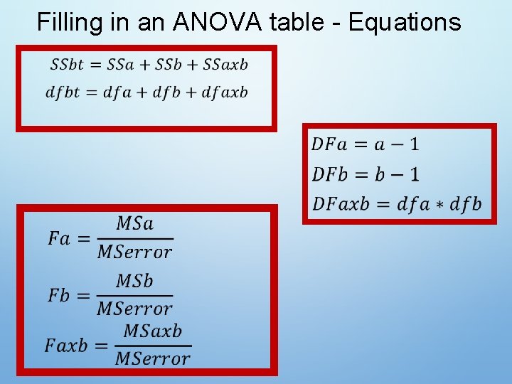
If we reject the omnibus null… SS and F for interaction: The Ax. B interaction is defined as the “extra” mean differences not accounted for by the main effects • SSAx. B= SSbetween treatments – SSA-SSB • df. Ax. B= dfbetween treatments – df. A-df. B Between Treatment Variability SSbetween treatment • F=MSAx. B/MSE Factor A Variability SSA Factor B Variability SSB Interaction Variability SSAB

Source SS df Between [(T 2/n)] - G 2/N ab-1 Within/ Error Total Source [ (x 2) – (T 2/n)] N-ab (x 2) - G 2/N MS F SSBT/dfbt MSBT/MS E SSE/df. E N-1 SS df MS F Factor A (Ta 2/n) - G 2/N a-1 SSA/dfa MSA/MSE Factor B (Tb 2/n) - G 2/N b-1 SSB/dfb MSB/MSE SSAB/dfab MSAx. B/MSE Interact SSBT-SSA-SSB dfbt– df. A-df. B

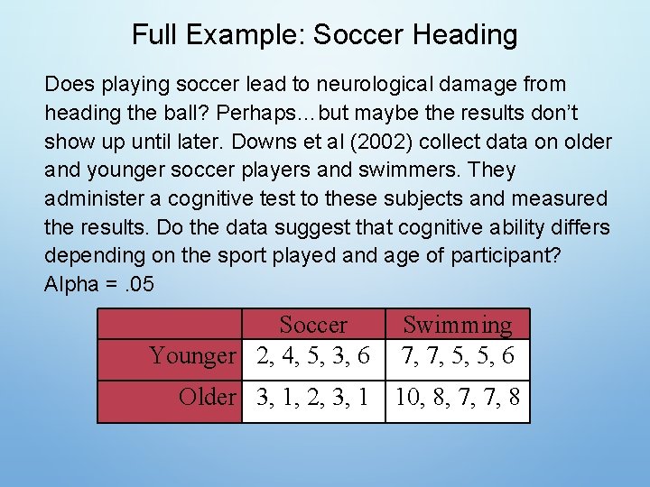
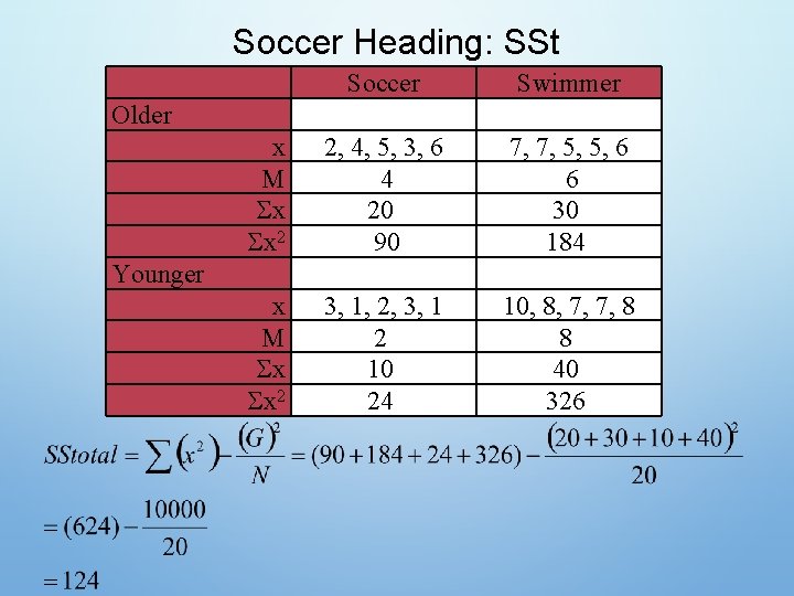
Full Example: Soccer Heading Does playing soccer lead to neurological damage from heading the ball? Perhaps…but maybe the results don’t show up until later. Downs et al (2002) collect data on older and younger soccer players and swimmers. They administer a cognitive test to these subjects and measured the results. Do the data suggest that cognitive ability differs depending on the sport played and age of participant? Alpha =. 05 Soccer Younger 2, 4, 5, 3, 6 Swimming 7, 7, 5, 5, 6 Older 3, 1, 2, 3, 1 10, 8, 7, 7, 8

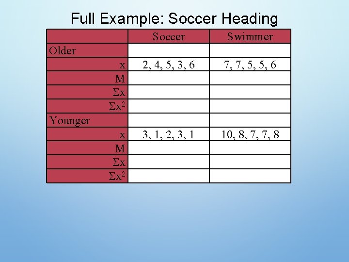
Full Example: Soccer Heading Soccer Swimmer x M x x 2 2, 4, 5, 3, 6 7, 7, 5, 5, 6 x M x x 2 3, 1, 2, 3, 1 10, 8, 7, 7, 8 Older Younger

Soccer Heading: SSt Soccer Swimmer x M x x 2 2, 4, 5, 3, 6 4 20 90 7, 7, 5, 5, 6 6 30 184 x M x x 2 3, 1, 2, 3, 1 2 10 24 10, 8, 7, 7, 8 8 40 326 Older Younger

Soccer Heading: SSbt Soccer Swimmer x M x x 2 2, 4, 5, 3, 6 4 20 90 7, 7, 5, 5, 6 6 30 184 x M x x 2 3, 1, 2, 3, 1 2 10 24 10, 8, 7, 7, 8 8 40 326 Older Younger

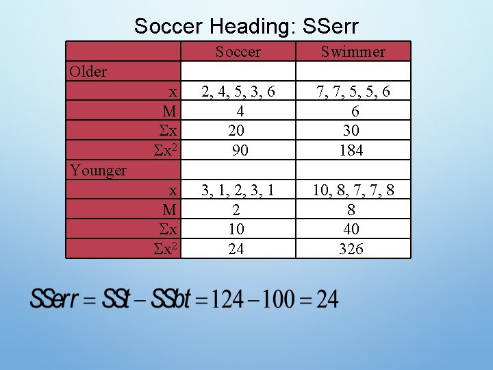
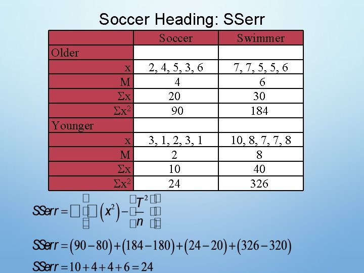
Soccer Heading: SSerr Soccer Swimmer x M x x 2 2, 4, 5, 3, 6 4 20 90 7, 7, 5, 5, 6 6 30 184 x M x x 2 3, 1, 2, 3, 1 2 10 24 10, 8, 7, 7, 8 8 40 326 Older Younger

Soccer Heading: SSerr Soccer Swimmer x M x x 2 2, 4, 5, 3, 6 4 20 90 7, 7, 5, 5, 6 6 30 184 x M x x 2 3, 1, 2, 3, 1 2 10 24 10, 8, 7, 7, 8 8 40 326 Older Younger

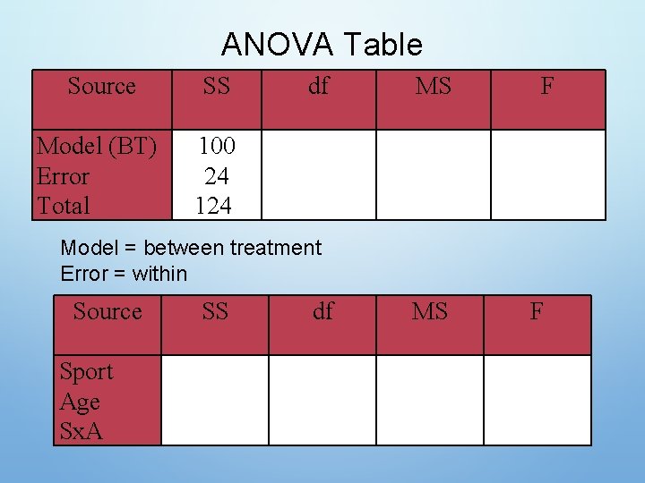
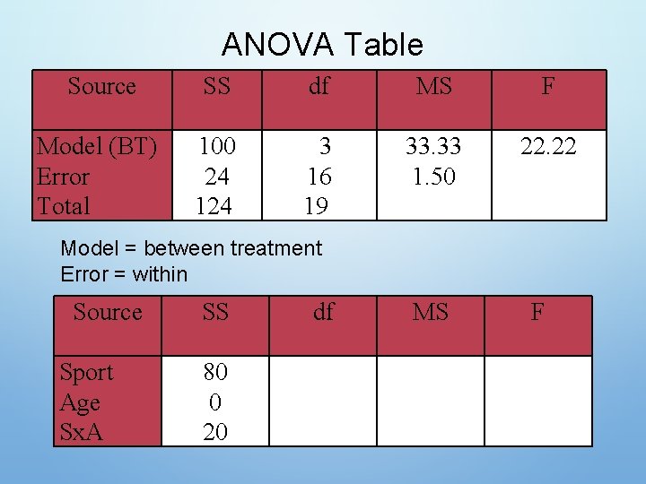
ANOVA Table Source SS Model (BT) Error Total 100 24 124 df MS F Model = between treatment Error = within Source Sport Age Sx. A SS df MS F

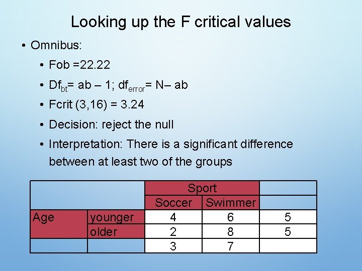
Looking up the F critical values • Omnibus: • Fob =22. 22 • Dfbt= ab – 1; dferror= N– ab • Fcrit (3, 16) = 3. 24 • Decision: reject the null • Interpretation: There is a significant difference between at least two of the groups Age younger older Sport Soccer Swimmer 4 6 2 8 3 7 5 5

ANOVA Table Source SS df MS F Model (BT) Error Total 100 24 124 3 16 19 33. 33 1. 50 22. 22 Model = between treatment Error = within Source Sport Age Sx. A SS df MS F

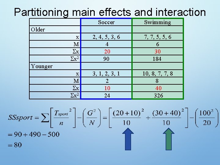
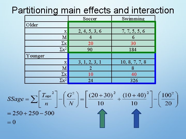
Partitioning main effects and interaction Soccer Swimming x M x x 2 2, 4, 5, 3, 6 4 20 90 7, 7, 5, 5, 6 6 30 184 x M x x 2 3, 1, 2, 3, 1 2 10 24 10, 8, 7, 7, 8 8 40 326 Older Younger

Partitioning main effects and interaction Soccer Swimming x M x x 2 2, 4, 5, 3, 6 4 20 90 7, 7, 5, 5, 6 6 30 184 x M x x 2 3, 1, 2, 3, 1 2 10 24 10, 8, 7, 7, 8 8 40 326 Older Younger

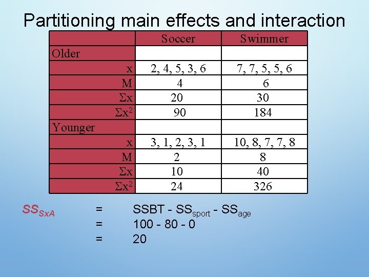
Partitioning main effects and interaction Soccer Swimmer x M x x 2 2, 4, 5, 3, 6 4 20 90 7, 7, 5, 5, 6 6 30 184 x M x x 2 3, 1, 2, 3, 1 2 10 24 10, 8, 7, 7, 8 8 40 326 Older Younger SSSx. A = = = SSBT - SSsport - SSage 100 - 80 - 0 20

ANOVA Table Source SS df MS F Model (BT) Error Total 100 24 124 3 16 19 33. 33 1. 50 22. 22 Model = between treatment Error = within Source Sport Age Sx. A SS 80 0 20 df MS F

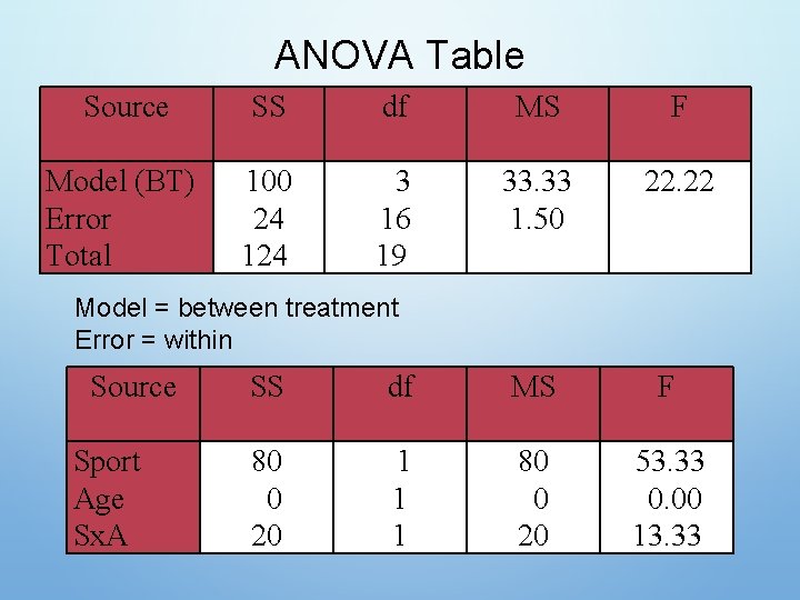
ANOVA Table Source SS df MS F Model (BT) Error Total 100 24 124 3 16 19 33. 33 1. 50 22. 22 Model = between treatment Error = within Source Sport Age Sx. A SS df MS F 80 0 20 1 1 1 80 0 20 53. 33 0. 00 13. 33

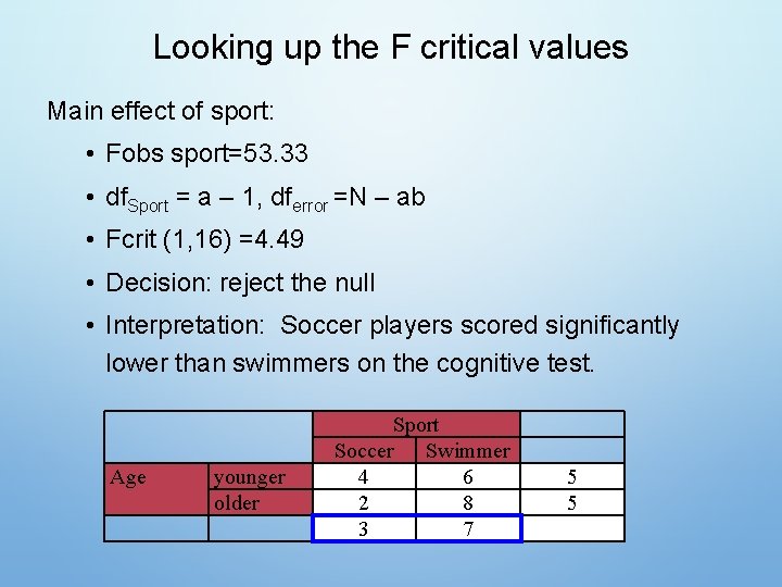
Looking up the F critical values Main effect of sport: • Fobs sport=53. 33 • df. Sport = a – 1, dferror =N – ab • Fcrit (1, 16) =4. 49 • Decision: reject the null • Interpretation: Soccer players scored significantly lower than swimmers on the cognitive test. Age younger older Sport Soccer Swimmer 4 6 2 8 3 7 5 5

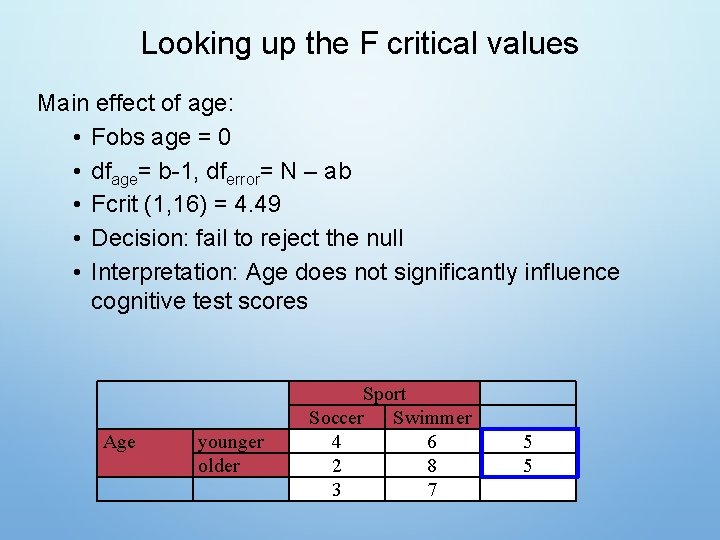
Looking up the F critical values Main effect of age: • Fobs age = 0 • dfage= b-1, dferror= N – ab • Fcrit (1, 16) = 4. 49 • Decision: fail to reject the null • Interpretation: Age does not significantly influence cognitive test scores Age younger older Sport Soccer Swimmer 4 6 2 8 3 7 5 5

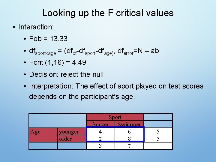
Looking up the F critical values • Interaction: • Fob = 13. 33 • dfsportxage = (dfbt-dfsport-dfage), dferror=N – ab • Fcrit (1, 16) = 4. 49 • Decision: reject the null • Interpretation: The effect of sport played on test scores depends on the participant’s age. Age younger older Sport Soccer Swimmer 4 6 2 8 3 7 5 5

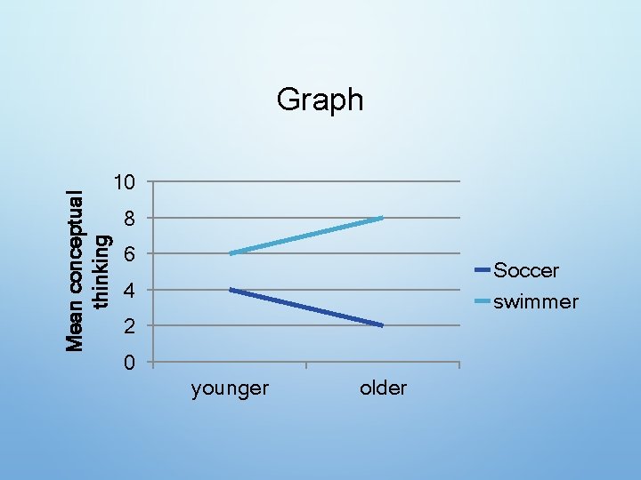
Mean conceptual thinking Graph 10 8 6 Soccer swimmer 4 2 0 younger older

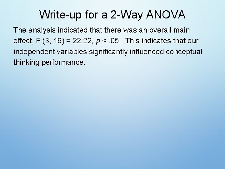
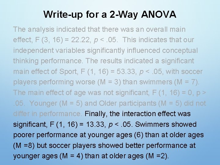
Write-up for a 2 -Way ANOVA The analysis indicated that there was an overall main effect, F (3, 16) = 22. 22, p <. 05. This indicates that our independent variables significantly influenced conceptual thinking performance.

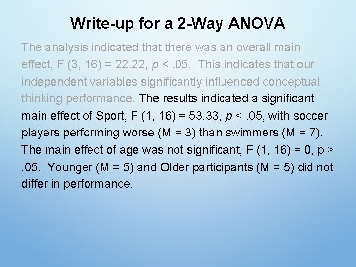
Write-up for a 2 -Way ANOVA The analysis indicated that there was an overall main effect, F (3, 16) = 22. 22, p <. 05. This indicates that our independent variables significantly influenced conceptual thinking performance. The results indicated a significant main effect of Sport, F (1, 16) = 53. 33, p <. 05, with soccer players performing worse (M = 3) than swimmers (M = 7). The main effect of age was not significant, F (1, 16) = 0, p >. 05. Younger (M = 5) and Older participants (M = 5) did not differ in performance.

Write-up for a 2 -Way ANOVA The analysis indicated that there was an overall main effect, F (3, 16) = 22. 22, p <. 05. This indicates that our independent variables significantly influenced conceptual thinking performance. The results indicated a significant main effect of Sport, F (1, 16) = 53. 33, p <. 05, with soccer players performing worse (M = 3) than swimmers (M = 7). The main effect of age was not significant, F (1, 16) = 0, p >. 05. Younger (M = 5) and Older participants (M = 5) did not differ in performance. Finally, the interaction effect was significant, F (1, 16) = 13. 33, p <. 05. Swimmers showed poorer performance at younger ages (6) than at older ages (M =8) but soccer players showed better performance at younger ages (M = 4) than at older ages (M =2).

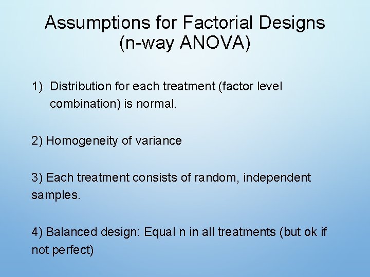
Assumptions for Factorial Designs (n-way ANOVA) 1) Distribution for each treatment (factor level combination) is normal. 2) Homogeneity of variance 3) Each treatment consists of random, independent samples. 4) Balanced design: Equal n in all treatments (but ok if not perfect)

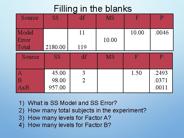
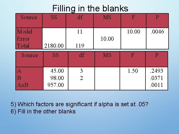
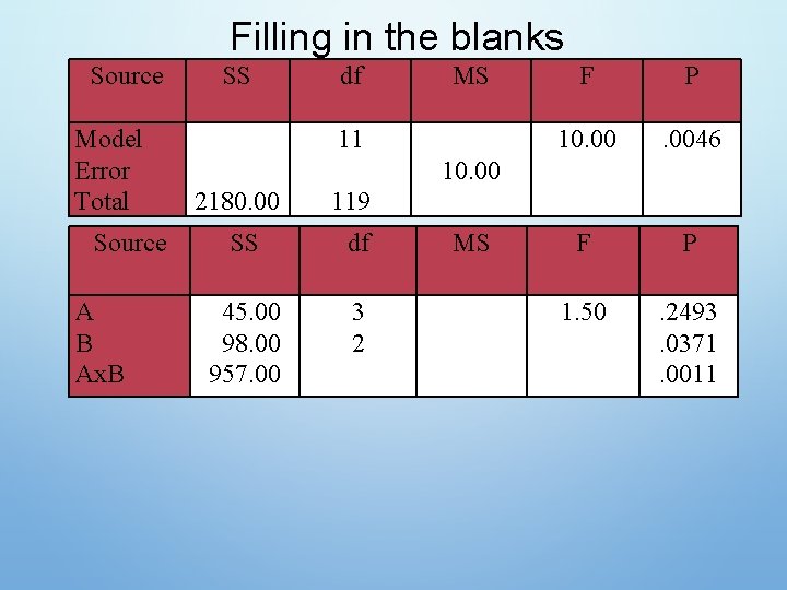
Filling in the blanks Source Model Error Total Source A B Ax. B 1) 2) 3) 4) SS df MS 11 F P 10. 0046 F P 1. 50 . 2493. 0371. 0011 10. 00 2180. 00 119 SS df 45. 00 98. 00 957. 00 3 2 MS What is SS Model and SS Error? How many total subjects in the experiment? How many levels for Factor A? How many levels for Factor B?

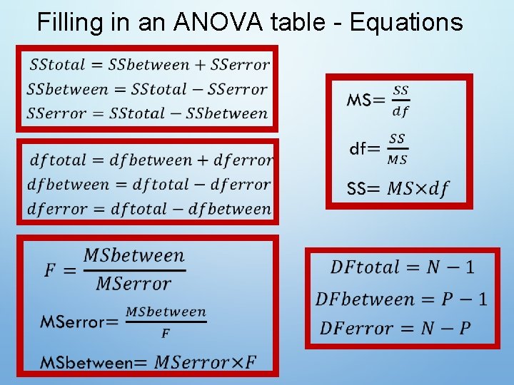
Filling in an ANOVA table - Equations

Filling in an ANOVA table - Equations

Filling in the blanks Source Model Error Total Source A B Ax. B 1) 2) 3) 4) SS df MS 11 F P 10. 0046 F P 1. 50 . 2493. 0371. 0011 10. 00 2180. 00 119 SS df 45. 00 98. 00 957. 00 3 2 MS What is SS Model and SS Error? How many total subjects in the experiment? How many levels for Factor A? How many levels for Factor B?

Filling in the blanks Source Model Error Total Source A B Ax. B SS df MS 11 F P 10. 0046 F P 1. 50 . 2493. 0371. 0011 10. 00 2180. 00 119 SS df 45. 00 98. 00 957. 00 3 2 MS 5) Which factors are significant if alpha is set at. 05? 6) Fill in the other blanks

Filling in the blanks Source Model Error Total Source A B Ax. B SS df MS 11 F P 10. 0046 F P 1. 50 . 2493. 0371. 0011 10. 00 2180. 00 119 SS df 45. 00 98. 00 957. 00 3 2 MS

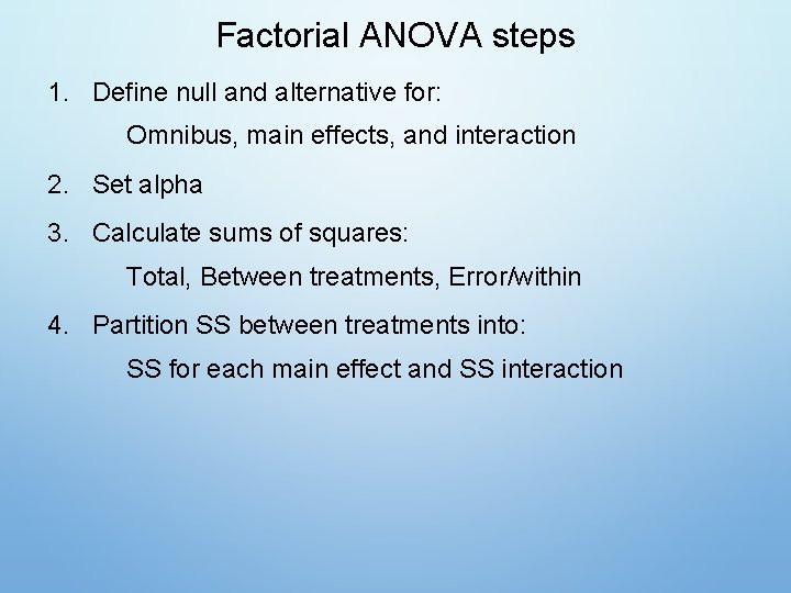
Factorial ANOVA steps 1. Define null and alternative for: Omnibus, main effects, and interaction 2. Set alpha 3. Calculate sums of squares: Total, Between treatments, Error/within 4. Partition SS between treatments into: SS for each main effect and SS interaction

Factorial ANOVA steps 5. Calculate mean squares and F ratios: omnibus, main effects, interaction 6. Identify F critical values for: omnibus, main effects, interaction 7. Make decisions about rejecting the null 8. Interpret results

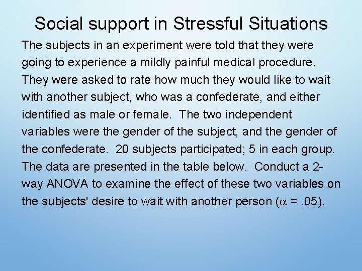
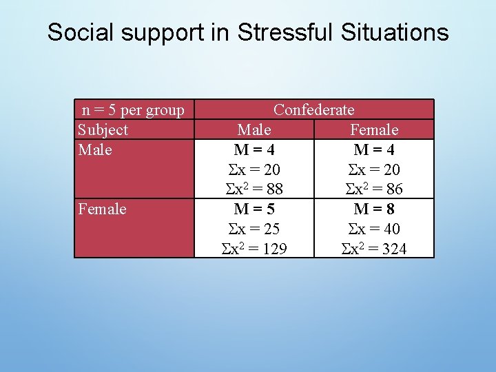
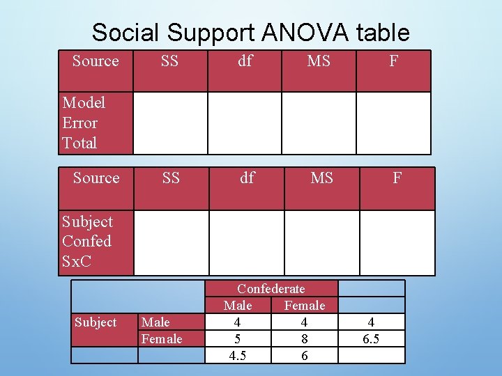
Social support in Stressful Situations The subjects in an experiment were told that they were going to experience a mildly painful medical procedure. They were asked to rate how much they would like to wait with another subject, who was a confederate, and either identified as male or female. The two independent variables were the gender of the subject, and the gender of the confederate. 20 subjects participated; 5 in each group. The data are presented in the table below. Conduct a 2 way ANOVA to examine the effect of these two variables on the subjects' desire to wait with another person ( =. 05).

Social support in Stressful Situations n = 5 per group Subject Male Female Confederate Male Female M=4 x = 20 x 2 = 88 x 2 = 86 M=5 M=8 x = 25 x = 40 x 2 = 129 x 2 = 324

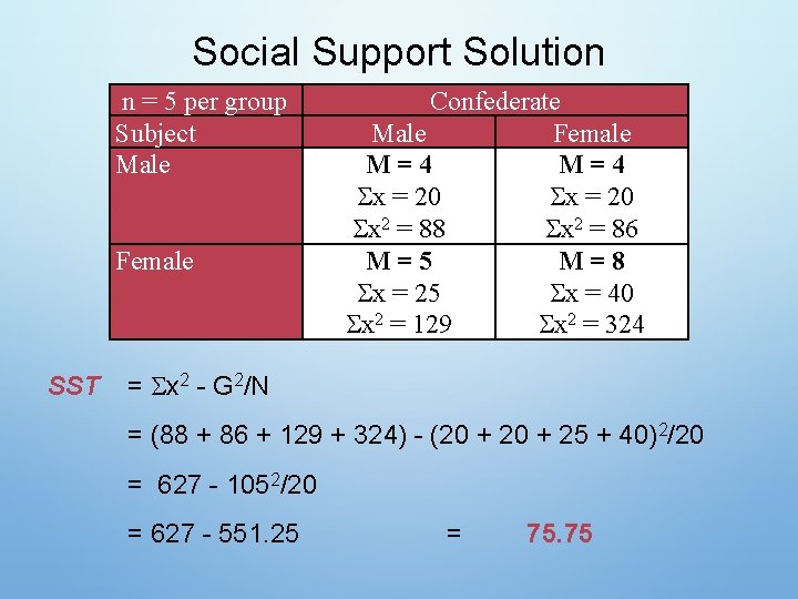
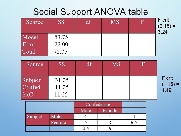
Social Support Solution n = 5 per group Subject Male Female SST Confederate Male Female M=4 x = 20 x 2 = 88 x 2 = 86 M=5 M=8 x = 25 x = 40 x 2 = 129 x 2 = 324 = x 2 - G 2/N = (88 + 86 + 129 + 324) - (20 + 25 + 40)2/20 = 627 - 1052/20 = 627 - 551. 25 = 75. 75

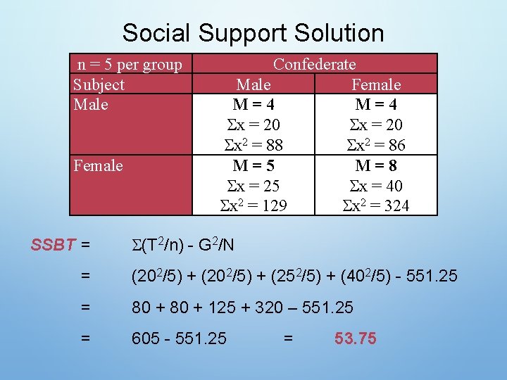
Social Support Solution n = 5 per group Subject Male Female SSBT = Confederate Male Female M=4 x = 20 x 2 = 88 x 2 = 86 M=5 M=8 x = 25 x = 40 x 2 = 129 x 2 = 324 (T 2/n) - G 2/N = (202/5) + (252/5) + (402/5) - 551. 25 = 80 + 125 + 320 – 551. 25 = 605 - 551. 25 = 53. 75

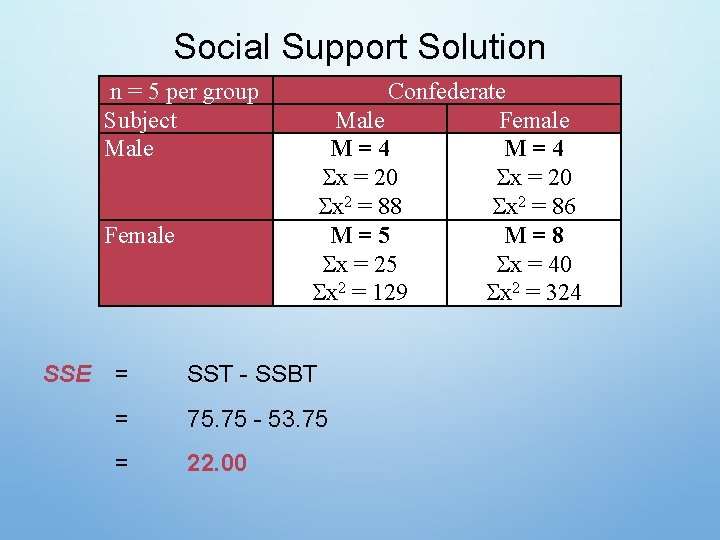
Social Support Solution n = 5 per group Subject Male Female SSE Confederate Male Female M=4 x = 20 x 2 = 88 x 2 = 86 M=5 M=8 x = 25 x = 40 x 2 = 129 x 2 = 324 = SST - SSBT = 75. 75 - 53. 75 = 22. 00

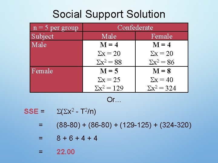
Social Support Solution n = 5 per group Subject Male Female Confederate Male Female M=4 x = 20 x 2 = 88 x 2 = 86 M=5 M=8 x = 25 x = 40 x 2 = 129 x 2 = 324 Or… SSE = ( x 2 - T 2/n) = (88 -80) + (86 -80) + (129 -125) + (324 -320) = 8+6+4+4 = 22. 00

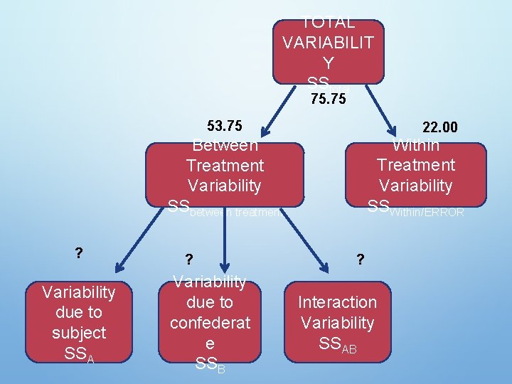
TOTAL VARIABILIT Y SStotal 75. 75 53. 75 22. 00 Within Treatment Variability SSWithin/ERROR Between Treatment Variability SSbetween treatment ? Variability due to subject SSA ? Variability due to confederat e SSB ? Interaction Variability SSAB

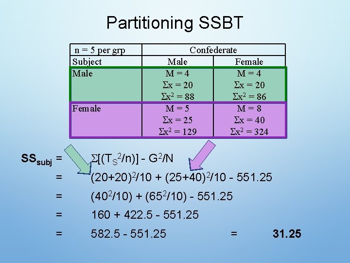
Partitioning SSBT n = 5 per grp Subject Male Female SSsubj = Confederate Male Female M=4 x = 20 x 2 = 88 x 2 = 86 M=5 M=8 x = 25 x = 40 x 2 = 129 x 2 = 324 [(TS 2/n)] - G 2/N = (20+20)2/10 + (25+40)2/10 - 551. 25 = (402/10) + (652/10) - 551. 25 = 160 + 422. 5 - 551. 25 = 582. 5 - 551. 25 = 31. 25

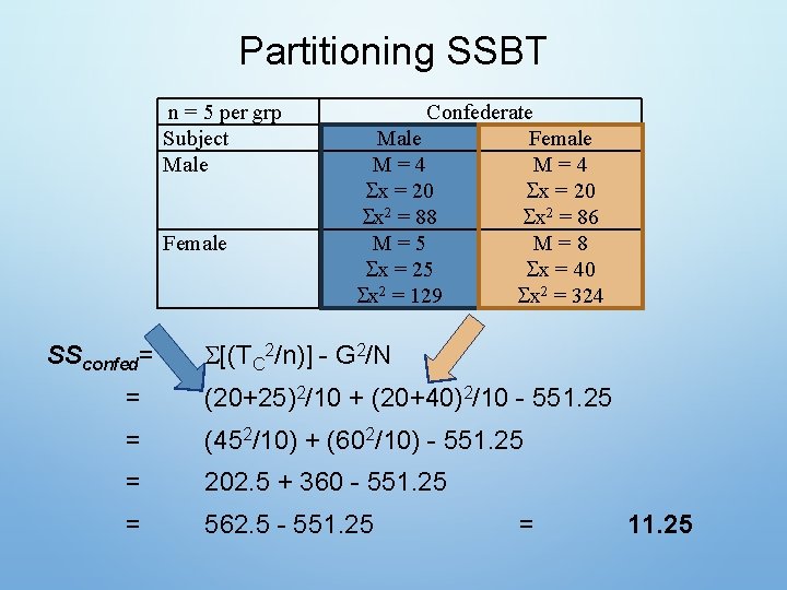
Partitioning SSBT n = 5 per grp Subject Male Female SSconfed= Confederate Male Female M=4 x = 20 x 2 = 88 x 2 = 86 M=5 M=8 x = 25 x = 40 x 2 = 129 x 2 = 324 [(TC 2/n)] - G 2/N = (20+25)2/10 + (20+40)2/10 - 551. 25 = (452/10) + (602/10) - 551. 25 = 202. 5 + 360 - 551. 25 = 562. 5 - 551. 25 = 11. 25

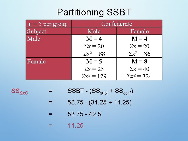
Partitioning SSBT n = 5 per group Subject Male Female SSSx. C Confederate Male Female M=4 x = 20 x 2 = 88 x 2 = 86 M=5 M=8 x = 25 x = 40 x 2 = 129 x 2 = 324 = SSBT - (SSsubj + SSconf) = 53. 75 - (31. 25 + 11. 25) = 53. 75 - 42. 5 = 11. 25

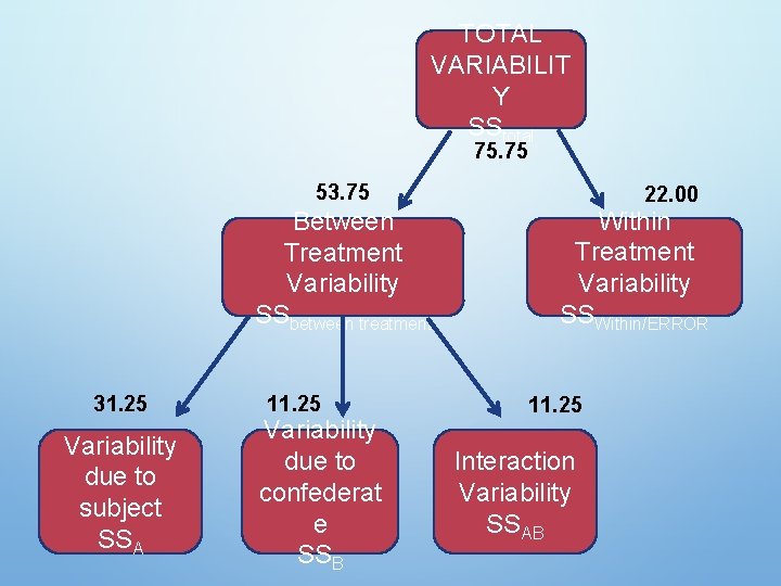
TOTAL VARIABILIT Y SStotal 75. 75 53. 75 Between Treatment Variability SSbetween treatment 31. 25 Variability due to subject SSA 11. 25 Variability due to confederat e SSB 22. 00 Within Treatment Variability SSWithin/ERROR 11. 25 Interaction Variability SSAB

Social Support ANOVA table Source SS df MS F Model Error Total Source Subject Confed Sx. C Subject Male Female Confederate Male Female 4 4 5 8 4. 5 6 4 6. 5

Social Support ANOVA table Source Model Error Total Source Subject Confed Sx. C Subject SS df MS F 53. 75 22. 00 75. 75 SS F crit (1, 16) = 4. 49 31. 25 11. 25 Male Female F crit (3, 16) = 3. 24 Confederate Male Female 4 4 5 8 4. 5 6 4 6. 5

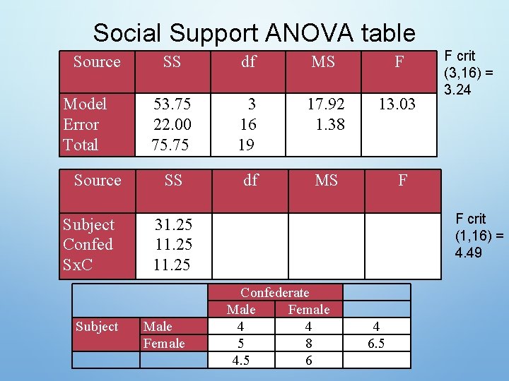
Social Support ANOVA table Source Model Error Total Source Subject Confed Sx. C Subject SS df MS F 53. 75 22. 00 75. 75 3 16 19 17. 92 1. 38 13. 03 SS df MS F F crit (1, 16) = 4. 49 31. 25 11. 25 Male Female F crit (3, 16) = 3. 24 Confederate Male Female 4 4 5 8 4. 5 6 4 6. 5

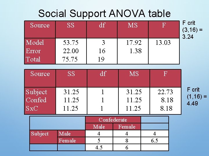
Social Support ANOVA table Source Model Error Total Source Subject Confed Sx. C Subject SS df MS F 53. 75 22. 00 75. 75 3 16 19 17. 92 1. 38 13. 03 SS df MS F 31. 25 11. 25 1 1 1 31. 25 11. 25 22. 73 8. 18 Male Female Confederate Male Female 4 4 5 8 4. 5 6 4 6. 5 F crit (3, 16) = 3. 24 F crit (1, 16) = 4. 49

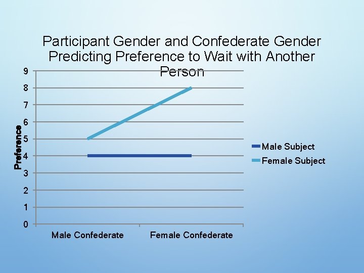
9 Participant Gender and Confederate Gender Predicting Preference to Wait with Another Person 8 Preference 7 6 5 Male Subject 4 Female Subject 3 2 1 0 Male Confederate Female Confederate

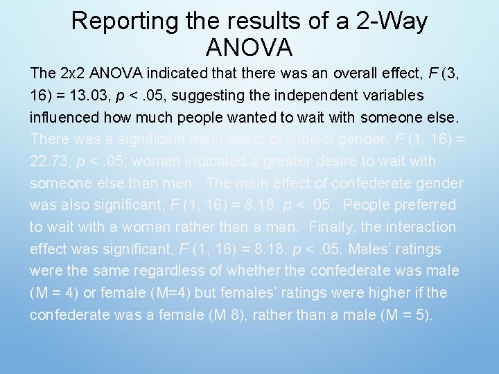
Reporting the results of a 2 -Way ANOVA The 2 x 2 ANOVA indicated that there was an overall effect, F (3, 16) = 13. 03, p <. 05, suggesting the independent variables influenced how much people wanted to wait with someone else. There was a significant main effect of subject gender, F (1, 16) = 22. 73, p <. 05; women indicated a greater desire to wait with someone else than men. The main effect of confederate gender was also significant, F (1, 16) = 8. 18, p <. 05. People preferred to wait with a woman rather than a man. Finally, the interaction effect was significant, F (1, 16) = 8. 18, p <. 05. Males’ ratings were the same regardless of whether the confederate was male (M = 4) or female (M=4) but females’ ratings were higher if the confederate was a female (M 8), rather than a male (M = 5).

Reporting the results of a 2 -Way ANOVA The 2 x 2 ANOVA indicated that there was an overall effect, F (3, 16) = 13. 03, p <. 05, suggesting the independent variables influenced how much people wanted to wait with someone else. There was a significant main effect of subject gender, F (1, 16) = 22. 73, p <. 05; women indicated a greater desire to wait with someone else than men. The main effect of confederate gender was also significant, F (1, 16) = 8. 18, p <. 05. People preferred to wait with a woman rather than a man. Finally, the interaction effect was significant, F (1, 16) = 8. 18, p <. 05. Males’ ratings were the same regardless of whether the confederate was male (M = 4) or female (M=4) but females’ ratings were higher if the confederate was a female (M 8), rather than a male (M = 5).

Reporting the results of a 2 -Way ANOVA The 2 x 2 ANOVA indicated that there was an overall effect, F (3, 16) = 13. 03, p <. 05, suggesting the independent variables influenced how much people wanted to wait with someone else. There was a significant main effect of subject gender, F (1, 16) = 22. 73, p <. 05; women indicated a greater desire to wait with someone else than men. The main effect of confederate gender was also significant, F (1, 16) = 8. 18, p <. 05. People preferred to wait with a woman rather than a man. Finally, the interaction effect was significant, F (1, 16) = 8. 18, p <. 05. Males’ ratings were the same regardless of whether the confederate was male (M = 4) or female (M=4) but females’ ratings were higher if the confederate was a female (M 8), rather than a male (M = 5).

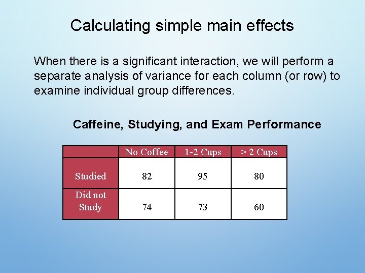
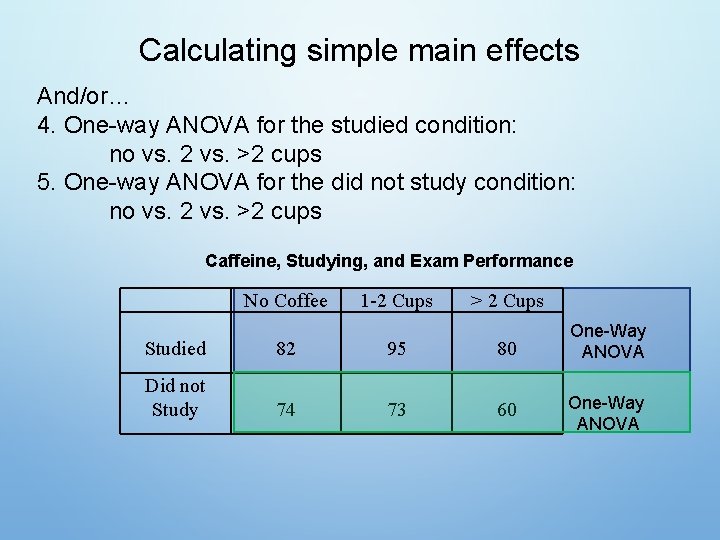
Calculating simple main effects When there is a significant interaction, we will perform a separate analysis of variance for each column (or row) to examine individual group differences. Caffeine, Studying, and Exam Performance No Coffee 1 -2 Cups > 2 Cups Studied 82 95 80 Did not Study 74 73 60

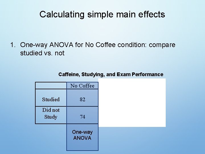
Calculating simple main effects 1. One-way ANOVA for No Coffee condition: compare studied vs. not Caffeine, Studying, and Exam Performance No Coffee 2 Cups > 2 Cups Studied 82 95 80 Did not Study 74 73 60 One-way ANOVA

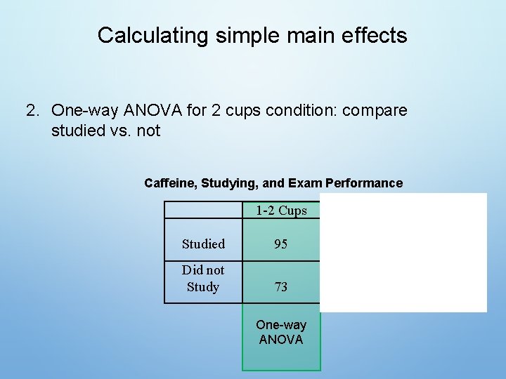
Calculating simple main effects 2. One-way ANOVA for 2 cups condition: compare studied vs. not Caffeine, Studying, and Exam Performance 1 -2 Cups > 2 Cups Studied 95 80 Did not Study 73 60 One-way ANOVA

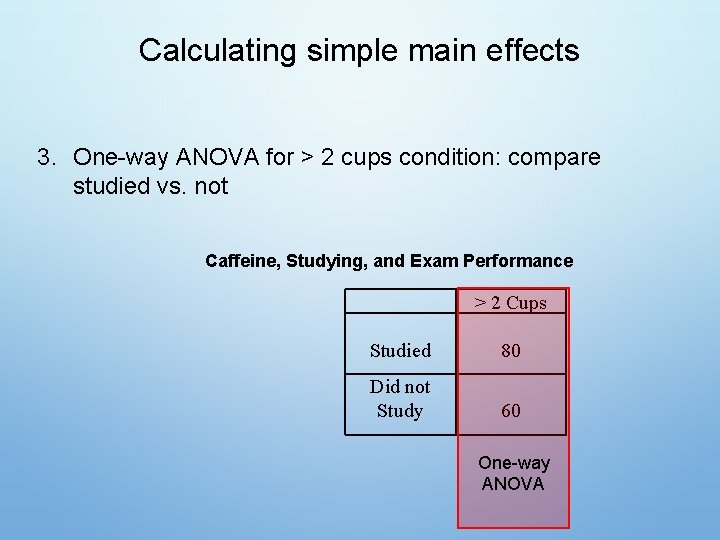
Calculating simple main effects 3. One-way ANOVA for > 2 cups condition: compare studied vs. not Caffeine, Studying, and Exam Performance > 2 Cups Studied 80 Did not Study 60 One-way ANOVA

Calculating simple main effects And/or… 4. One-way ANOVA for the studied condition: no vs. 2 vs. >2 cups 5. One-way ANOVA for the did not study condition: no vs. 2 vs. >2 cups Caffeine, Studying, and Exam Performance No Coffee 1 -2 Cups > 2 Cups Studied 82 95 80 One-Way ANOVA Did not Study 74 73 60 One-Way ANOVA

More practice with Interpretation

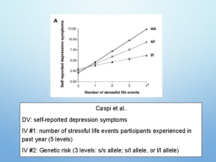
Caspi et al. . DV: self-reported depression symptoms IV #1: number of stressful life events participants experienced in past year (5 levels) IV #2: Genetic risk (3 levels: s/s allele; s/l allele, or l/l allele)

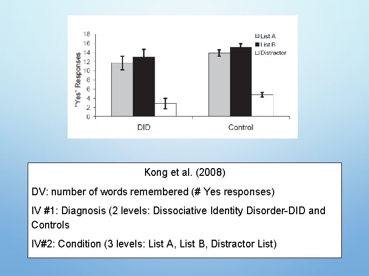
Kong et al. (2008) DV: number of words remembered (# Yes responses) IV #1: Diagnosis (2 levels: Dissociative Identity Disorder-DID and Controls IV#2: Condition (3 levels: List A, List B, Distractor List)

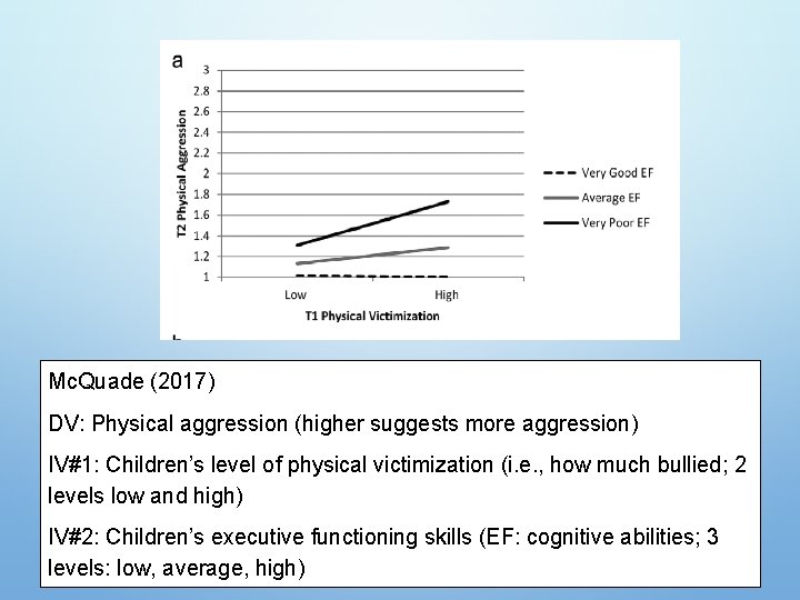
Mc. Quade (2017) DV: Physical aggression (higher suggests more aggression) IV#1: Children’s level of physical victimization (i. e. , how much bullied; 2 levels low and high) IV#2: Children’s executive functioning skills (EF: cognitive abilities; 3 levels: low, average, high)

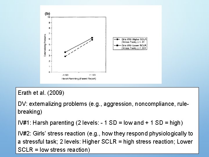
Erath et al. (2009) DV: externalizing problems (e. g. , aggression, noncompliance, rulebreaking) IV#1: Harsh parenting (2 levels: - 1 SD = low and + 1 SD = high) IV#2: Girls’ stress reaction (e. g. , how they respond physiologically to a stressful task; 2 levels: Higher SCLR = high stress reaction; Lower SCLR = low stress reaction)