Design Of Experiments Initial Random Designs AC Initial

Design Of Experiments. Initial Random Designs AC

Initial Designs • Body of literature is divided into mainly two classes • Factorial Designs • Think of a rectangular grid • Random Designs • Think of randomly picking points from the parameter space • Current Postulations (Needs more digging…) • Factorial Designs are superior in characterizing the sensitivity of a response variable (Y) to individual changes in the input variables (X) (also referred to as factors which themselves may have variability in experiments) • Random Designs are more efficient if the goal is to build a model to capture the mean response variable (Y) for given input variables (x) (in computer experiments there is often no distribution about these parameters, i. e. deterministic so this is often the choice for design of computer experiments) • We also note since the output of computer simulations is deterministic there is little to gain from the repetition of an input (since there is no distribution of the actual output)

Vocabulary of Design of Experiments • Terminology often used • Factors (constraints, dimensions, number of input variables) • p factors • Levels (unique values of a factor) • n levels (for LHD this is also the total number of design points) • Properties of a design • Space Filling • How concentrated is a sub-volume in the parameter space with design points • Good Projection Properties • How uniformly spread are the points for a given 1 d, 2 d …. p-1 projection of the p dimensional design space D ØIf nothing is known about the response a-priori to the design of the experiments it is desirable to maximize these properties

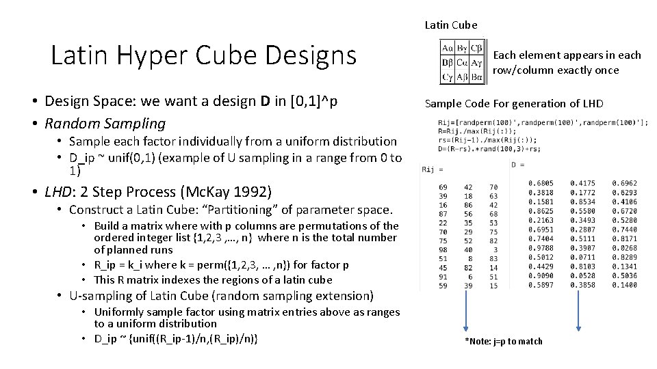
Latin Cube Latin Hyper Cube Designs • Design Space: we want a design D in [0, 1]^p • Random Sampling Each element appears in each row/column exactly once Sample Code For generation of LHD • Sample each factor individually from a uniform distribution • D_ip ~ unif(0, 1) (example of U sampling in a range from 0 to 1) • LHD: 2 Step Process (Mc. Kay 1992) • Construct a Latin Cube: “Partitioning” of parameter space. • Build a matrix where with p columns are permutations of the ordered integer list {1, 2, 3 , …, n} where n is the total number of planned runs • R_ip = k_i where k = perm({1, 2, 3, … , n}) for factor p • This R matrix indexes the regions of a latin cube • U-sampling of Latin Cube (random sampling extension) • Uniformly sample factor using matrix entries above as ranges to a uniform distribution • D_ip ~ {unif((R_ip-1)/n, (R_ip)/n)} *Note: j=p to match

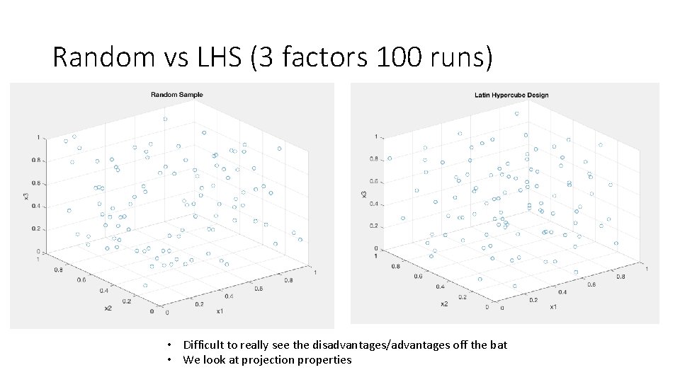
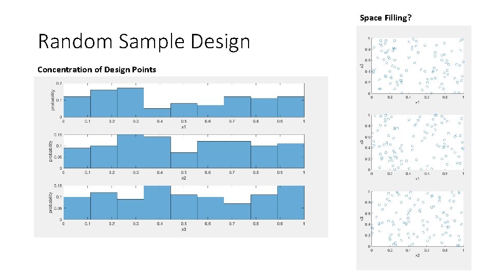
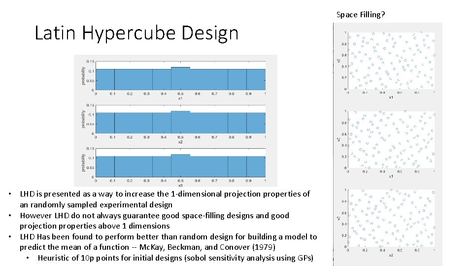
Random vs LHS (3 factors 100 runs) • Difficult to really see the disadvantages/advantages off the bat • We look at projection properties

Space Filling? Random Sample Design Concentration of Design Points

Latin Hypercube Design • LHD is presented as a way to increase the 1 -dimensional projection properties of an randomly sampled experimental design • However LHD do not always guarantee good space-filling designs and good projection properties above 1 dimensions • LHD Has been found to perform better than random design for building a model to predict the mean of a function -- Mc. Kay, Beckman, and Conover (1979) • Heuristic of 10 p points for initial designs (sobol sensitivity analysis using GPs) Space Filling?

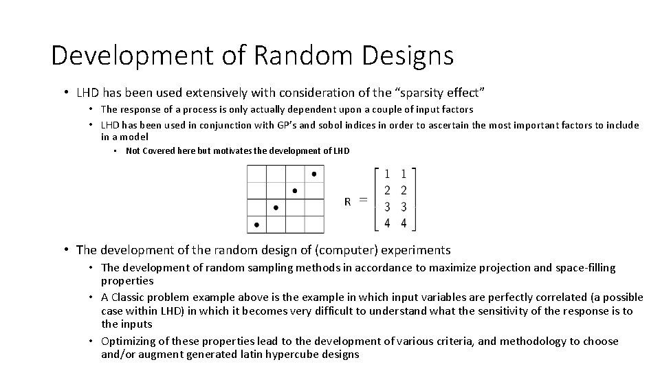
Development of Random Designs • LHD has been used extensively with consideration of the “sparsity effect” • The response of a process is only actually dependent upon a couple of input factors • LHD has been used in conjunction with GP’s and sobol indices in order to ascertain the most important factors to include in a model • Not Covered here but motivates the development of LHD R • The development of the random design of (computer) experiments • The development of random sampling methods in accordance to maximize projection and space-filling properties • A Classic problem example above is the example in which input variables are perfectly correlated (a possible case within LHD) in which it becomes very difficult to understand what the sensitivity of the response is to the inputs • Optimizing of these properties lead to the development of various criteria, and methodology to choose and/or augment generated latin hypercube designs

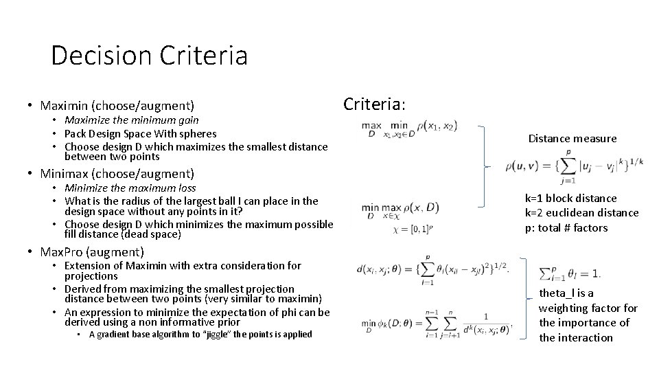
Decision Criteria • Maximin (choose/augment) • Maximize the minimum gain • Pack Design Space With spheres • Choose design D which maximizes the smallest distance between two points Criteria: Distance measure • Minimax (choose/augment) • Minimize the maximum loss • What is the radius of the largest ball I can place in the design space without any points in it? • Choose design D which minimizes the maximum possible fill distance (dead space) k=1 block distance k=2 euclidean distance p: total # factors • Max. Pro (augment) • Extension of Maximin with extra consideration for projections • Derived from maximizing the smallest projection distance between two points (very similar to maximin) • An expression to minimize the expectation of phi can be derived using a non informative prior • A gradient base algorithm to “jiggle” the points is applied theta_l is a weighting factor for the importance of the interaction

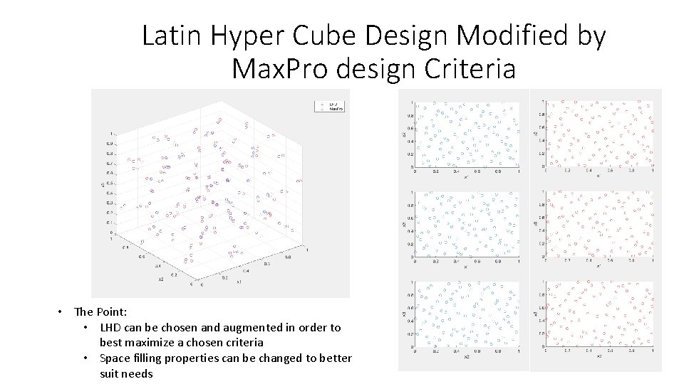
Latin Hyper Cube Design Modified by Max. Pro design Criteria • The Point: • LHD can be chosen and augmented in order to best maximize a chosen criteria • Space filling properties can be changed to better suit needs

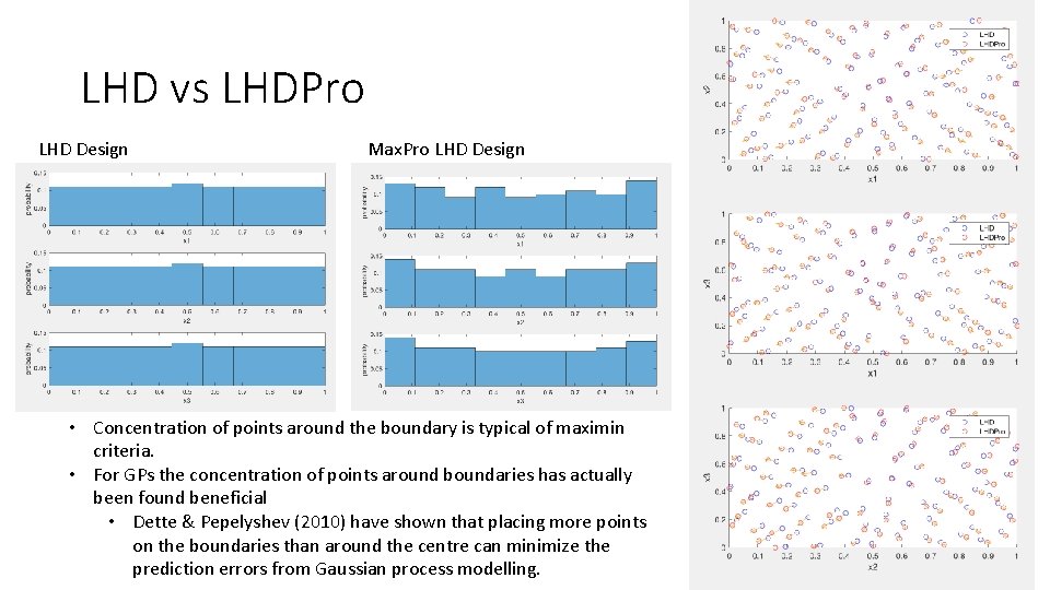
LHD vs LHDPro LHD Design Max. Pro LHD Design • Concentration of points around the boundary is typical of maximin criteria. • For GPs the concentration of points around boundaries has actually been found beneficial • Dette & Pepelyshev (2010) have shown that placing more points on the boundaries than around the centre can minimize the prediction errors from Gaussian process modelling.

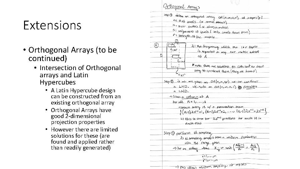
Extensions • Orthogonal Arrays (to be continued) • Intersection of Orthogonal arrays and Latin Hypercubes • A Latin Hypercube design can be constructed from an existing orthogonal array • Orthogonal Arrays have good 2 -dimensional projection properties • However there are limited solutions for these (are found applied rather than readily generated)

Example Problem (LANL Irradiated Problem) • Following…

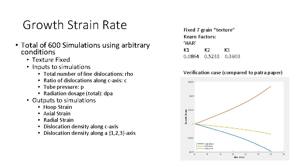
Growth Strain Rate • Total of 600 Simulations using arbitrary conditions • Texture Fixed • Inputs to simulations • • Total number of line dislocations: rho Ratio of dislocations along c-axis: c Tube pressure: p Radiation dosage (total): dpa • • • Hoop Strain Axial Strain Radial Strain Dislocation density along c-axis Dislocation density along a {1, 2, 3}-axis • Outputs to simulations Fixed 7 grain “texture” Kearn Factors: ‘HAR’ K 1 K 2 K 3 0. 0864 0. 5233 0. 3903 Verification case (compared to patra paper)

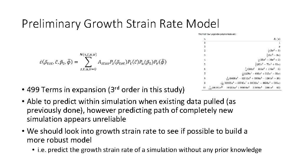
Preliminary Growth Strain Rate Model • 499 Terms in expansion (3 rd order in this study) • Able to predict within simulation when existing data pulled (as previously done), however predicting path of completely new simulation appears unreliable • We should look into growth strain rate to see if possible to build a more robust model • i. e. predict the growth strain rate of a simulation without any prior knowledge

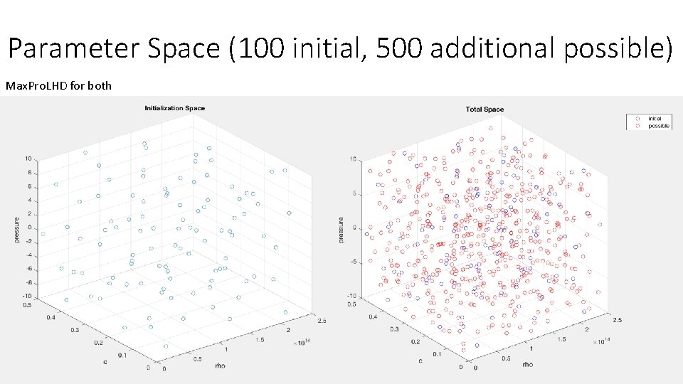
Parameter Space (100 initial, 500 additional possible) Max. Pro. LHD for both

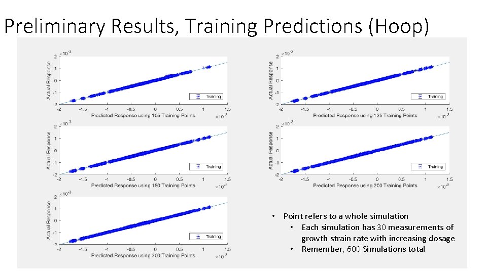
Preliminary Results, Training Predictions (Hoop) • Point refers to a whole simulation • Each simulation has 30 measurements of growth strain rate with increasing dosage • Remember, 600 Simulations total

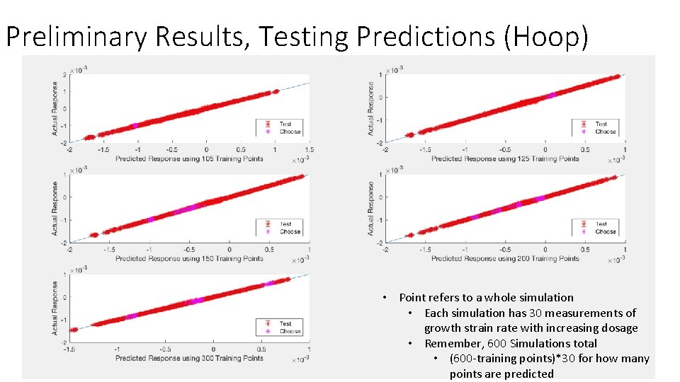
Preliminary Results, Testing Predictions (Hoop) • Point refers to a whole simulation • Each simulation has 30 measurements of growth strain rate with increasing dosage • Remember, 600 Simulations total • (600 -training points)*30 for how many points are predicted

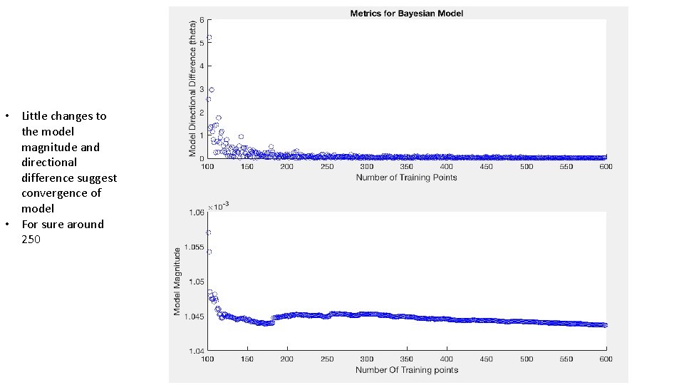
• Little changes to the model magnitude and directional difference suggest convergence of model • For sure around 250

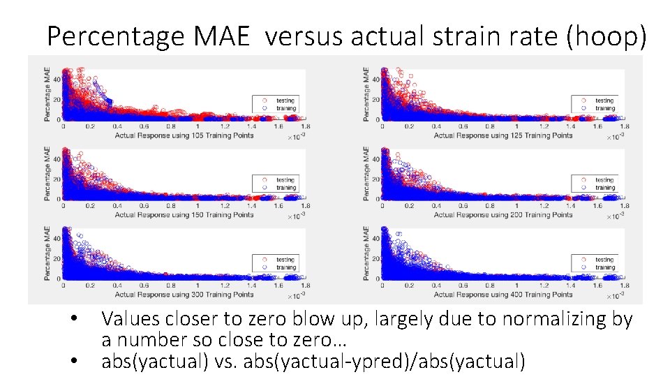
Percentage MAE versus actual strain rate (hoop) • • Values closer to zero blow up, largely due to normalizing by a number so close to zero… abs(yactual) vs. abs(yactual-ypred)/abs(yactual)