Other ANOVA designs Twoway ANOVA Chapter 11 Twoway

Other ANOVA designs Two-way ANOVA Chapter 11

Two-way ANOVA • In this chapter – Randomized block design – Factorial design

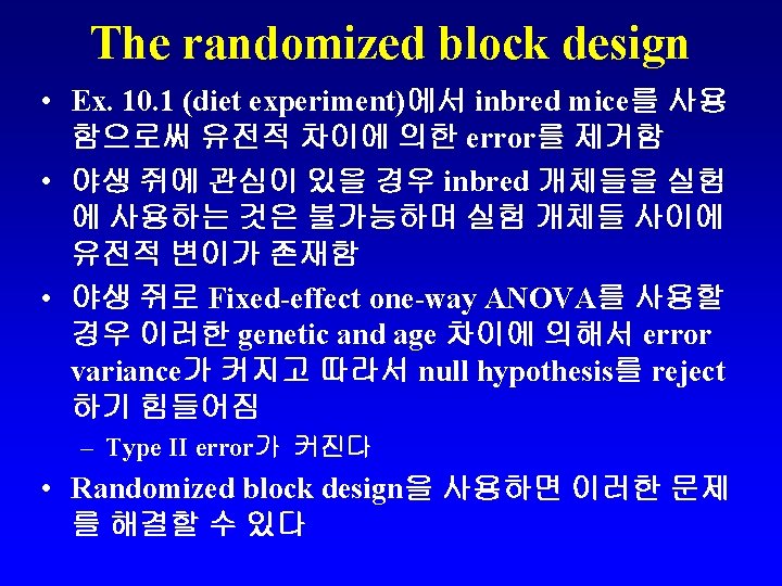
The randomized block design • Error variance를 분리해내기를 원하는 특성에 따라 실험개체들을 grouping (blocked) 한다 • Ex. 야생 쥐의 경우 litters (한배의 새끼)에 따라 grouping 한다 – Same litter의 경우 유전적으로 유사하고 same age 이므로 • 따라서 이 실험의 경우 실험대상 쥐들은 두 기준 (criteria)에 의해 분류됨 – Diet and litter – 각 diet and litter combination에 하나의 실험 개체가 존재 (no replication) – Two-way ANOVA without replication이라 부른다 – Mixed effects model • Diet: fixed factor; Litter: random factor

The randomized block design Variance (분산): -1. Total variance -2. Black (little)에 의한 분산 -3. Treatments (diets)에 의한 분산 -4. Error variance (오차분산)

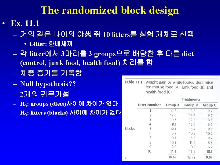
The randomized block design • • Calculation steps 1. 각 행 (row)의 값을 합함 (Σxr) 2. 각 열 (column)의 값을 합함 (Σxc) 3. column total 이나 row total을 계산, 두 값이 동일 함 (Σxt) • 4. 각 행의 합을 제곱 {(Σxr)2}; 제곱한 값을 다 합한 후 treatments (columns)의 수로 나눔 Σ(Σxr)2 / c – In this case: Σ(Σxr)2 / c = (1197. 16 + 1296. 0 + …+ 1232. 01)/3 = 3553. 27 • 5. 각 열의 합을 제곱: {(Σxc)2}; 제곱한 값을 다 합한 후 rows (blocks)의 수로 나눔: Σ(Σxc)2 / r – In this case: Σ(Σxc)2 / r = (11384. 89 + 16358. 41 + 8226. 49)/10 = 3596. 98

The randomized block design • Calculation steps • 6. 모든 observations을 제곱한 후 합함: Σx 2 t – (11. 8)2 + (12)2 + …. . + (10. 1)2 = 3631. 47 • 7. grand total을 제곱한 후 total observations으로 나 눔: (Σxt)2 / nt – (325. 30)2 / 30 = 3527. 336 – Correction term

The randomized block design • Total sum of square (SSt: 6 – 7) – Σx 2 t - (Σxt)2 / nt – 3631. 47 – 3527. 336 = 104. 134 • Sum of square for treatments (columns) (SSc: 5 – 7) – Σ(Σxc)2 / r - (Σxt)2 / nt – 3596. 98 – 3527. 336 = 69. 643 • Sum of square for blocks (rows) (SSr: 4 – 7) – Σ(Σxr)2 / c - (Σxt)2 / nt – 3553. 27 – 3527. 336 = 25. 934 • Error sum of square – SSe = SSt - SSc - SSr – 104. 134 – 69. 643 – 25. 934 = 8. 557

The randomized block design • Total degree of freedom (dft: nt – 1) – 30 - 1 = 29 • Treatments (columns) 자유도 (dfc: columns – 1) – 3– 1=2 • Blocks (rows) 자유도 (dfr: rows – 1) – 10 – 1 = 9 • Error degree of freedom (dfe = dft - dfc - dfr) – 29 – 2 – 9 = 18

The randomized block design • ANOVA table • For diet treatments – – – Critical F value in table A. 6 (α=0. 05, df = 2, 18) F (df = 2, 15) = 3. 68 Calculated F (73. 25)가 critical F value보다 훨씬 크다 따라서 null hypothesis를 reject 결론: diets 가 체중증가에 유의하게 영향을 미친다

The randomized block design • For blocks – – – Critical F value in table A. 6 (α=0. 05, df = 9, 18) F (df = 9, 15) = 2. 59 Calculated F (6. 06)가 critical F value보다 훨씬 크다 따라서 second null hypothesis를 reject 결론: litters에 따라 차이가 있음 • litters에 의한 error variance가 randomized block design을 사용함으로써 분리되어짐 • Randomized block ANOVA로는 treatments와 blocks 사이의 interaction (교호작용)을 알 수 없다 – Interaction: treatments가 blocks 에 따라 따르게 영향을 미 칠 경우, 또는 combined effects of the treatments and blocks 이 개개의 treatments와 blocks effects의 합과 다를 경우 – Two-way factorial design으로 interaction 을 알 수 있다

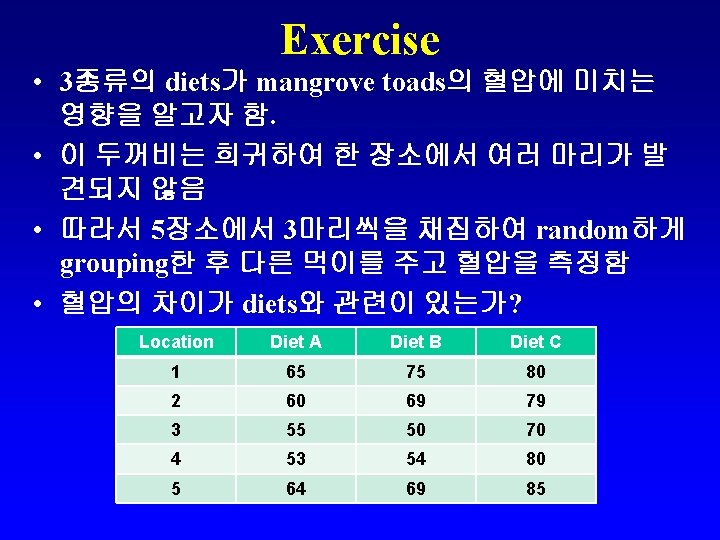
The randomized block design • 각행의 합 – 220, 208, 175, 187, 218 – 합의 제곱의 합 Location Diet A Diet B Diet C 1 65 75 80 2 60 69 79 3 55 50 70 4 53 54 80 5 64 69 85 • 48400+43264+30625+34969+47524 = 204782 • 각열의 합 – 297, 317, 394 – 합의 제곱의 합 • 88209+100489+155236 = 343934 • Correction term – (Σxt)2 / nt = 1016064/15 = 67737. 6 • Σx 2 t – 69484

The randomized block design Location Diet A Diet B Diet C • Total sum of square (SSt) – Σx 2 t - (Σxt)2 / nt – 69484 – 67737. 6 = 1746. 4 • Sum of square for treatments (columns) (SSc) – Σ(Σxc)2 / r - (Σxt)2 / nt – 17641. 8+20097. 8+31047. 2 – 67737. 6 = 1049. 2 • Sum of square for blocks (rows) (SSr) – Σ(Σxr)2 / c - (Σxt)2 / nt – 68260. 67 – 67737. 6 = 523. 07 • Error sum of square – SSe = SSt - SSc - SSr – 1746. 4 – 1049. 2 – 523. 07 = 174. 13 sum 1 65 75 80 220 2 60 69 79 208 3 55 50 70 175 4 53 54 80 187 5 64 69 85 218 297 317 394

The randomized block design • Total degree of freedom (dft: nt – 1) – 15 - 1 = 14 • Treatments (columns) 자유도 (dfc: columns – 1) – 3– 1=2 • Blocks (rows) 자유도 (dfr: rows – 1) – 5– 1=4 • Error degree of freedom (dfe = dft - dfc - dfr) – 14 – 2 – 4 = 8

The randomized block design • ANOVA table Source SS df MS F Diets 1049. 2 2 524. 6 24. 1 Blocks (location) 523. 07 4 130. 77 6. 01 Error 174. 13 8 21. 77 Total 1746. 4 14 • For diet treatments – – – Critical F value in table A. 6 (α=0. 05, df = 2, 8) F (df = 2, 8) = 4. 46 Calculated F (24. 1)가 critical F value보다 훨씬 크다 따라서 null hypothesis를 reject 결론: diets 가 두꺼비의 혈압에 유의하게 영향을 미친다

The randomized block design • ANOVA table Source SS df MS F Diets 1049. 2 2 524. 6 24. 1 Blocks (location) 523. 07 4 130. 77 6. 01 Error 174. 13 8 21. 77 Total 1746. 4 14 • For locations – – – Critical F value in table A. 6 (α=0. 05, df = 4, 8) F (df = 4, 8) = 3. 84 Calculated F (6. 01)가 critical F value보다 크다 따라서 null hypothesis를 reject 결론: location에 따라 차이가 있다

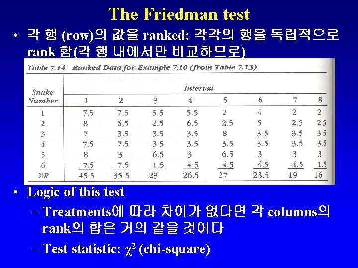
The Friedman test • Measurement scale? ? – Ordinal scale – 따라서 nonparametric test를 사용해야 함 – 각 개체들은 연속적으로 test 되었으므로 observations들은 independent 하지 않음: related sample

The Friedman test • k columns (8) and n rows (6) • ΣRi: sum of rank of a column • = 12/6× 8× 9 {(45. 5)2 + (35. 5)2 + (23)2 + (26. 5)2 + (27)2 + (23. 5)2 + (19)2 + (16)2} – (3× 6× 9) = 17. 44 • Degree of freedom: k – 1 = 8 – 1 = 7 • Critical chi-square value from Table A. 3: 14. 07 • Calculated chi-square value가 critical value보다 크다 • 자극시간에 따른 차이가 없다는 귀무가설을 reject • 결론: 뱀은 연속적인 자극에 약화되는 반응을 보인다

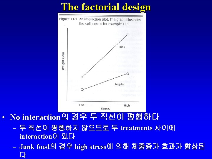
The factorial design • 많은 경우 두 factors (treatments)가 서로 상호작용 하여 각각의 factors의 합과 다른 effects를 줄 수 있 다 • In other word, treatments 들은 synergistically or antagonistically 영향을 미칠 수 있다 • Ex. 여러 종류의 약을 동시에 먹을 경우 유해한 영향 이 나타날 수 있다 • Treatments 사이에 interaction이 예견될 경우 factorial design을 사용

The factorial design • Both factors가 treatments로 고려됨 – Both treatments가 fixed effects 임 • Treatments 사이에 interaction이 있음 • 각 treatments의 combinations 은 replicated observations을 가짐 • Two-way ANOVA with replication이라 불림

The factorial design • Ex. 11. 2: a factorial design ANOVA – Diets 와 stress가 생쥐의 체중증가에 미치는 영향을 알고 자함 – Interaction effects도 알고자 함 – 32마리의 inbred mice를 실험동물로 사용 – Random 하게 4 groups으로 나눔 (8마리 씩) – Treatments • Diet: 2 treatments: junk food and control food • Stress: 2 treatments: High stress and low stress – Group 1: junk food + low stress – Group 2: junk food + high stress – Group 3: control food + low stress – Group 4: control food + high stress

The factorial design • Ex. 11. 2: a factorial design ANOVA – High stress: 매일 8시간 rap music – Low stress: 매일 8시간 classical music • Null hypothesis – 1. Effect of stress • H 0: Low = High vs Ha: Low ≠ High – 2. Effect of diet • H 0: Control = Junk food vs Ha: Control ≠ Junk food – 3. Interaction effect • H 0: no interaction vs Ha: interaction

The factorial design Variance (분산): -1. Total variance -2. Diet에 의한 분산 -3. Stress에 의한 분산 -4. Interaction에 의한 분산 -5. Error variance (오차분산)

The factorial design • Preliminary calculations as shown in Table 7. 11

The factorial design • Total sum of square (SSt) – Σx 2 t - (Σxt)2 / nt – 591136 – (4332)2/32 = 4691. 5 • Sum of square for stress (SSs) – (Σx. L)2 / n. L + (Σx. H)2 / n. H - (Σxt)2 / nt – (2058)2/16 + (2274)2/16 - (4332)2/32 = 1458 • Sum of square for diet (SSd) – (Σx. J)2 / n. J + (Σx. R)2 / n. R - (Σxt)2 / nt – (2278)2/16 + (2054)2/16 - (4332)2/32 = 1568

The factorial design • Sum of square for interaction (SSi) – (Σx. HR)2 / n. HR + (Σx. LR)2 / n. LR + (Σx. HJ)2 / n. HJ + (Σx. LJ)2 / n. LJ - (Σxt)2 / nt – SSs – SSd – (1060)2/8 + (998)2/8 + (1218)2/8 + (1056)2/8 - (4332)2/32 – 1458 – 1568 = 312. 5 • Error sum of square – SSe = SSt - (SSs + SSd + SSi) – 4561 – (1458 + 1568 + 312. 5) = 1222. 5

The factorial design • Degree of freedom for each main effect – Groups – 1 = 2 – 1 = 1 • Degree of freedom for interaction – dfstress * dfdiet = 1 * 1 = 1 • Total degree of freedom – nt – 1 = 32 – 1 = 31 • Error degree of freedom – dfe = dft - dfs - dfd - dfi = 31 – 1 – 1 = 28

The factorial design • • • Fstress = 1458 / 48. 32 = 30. 18 (df = 1, 28) Fdiet = 1568 / 48. 32 = 32. 46 (df = 1, 28) Finter = 312. 5 / 48. 32 = 6. 47 (df = 1, 28) Critical F value in Table A. 6 (α=0. 05, df = 1, 25): 4. 24 Calculated F value가 critical F value보다 크다 – 따라서 귀무가설을 reject • Stress 와 diet가 체중증가에 영향을 미치며 두 factors 사이에 interaction이 있다

Homework • 45마리의 guppy 암컷을 9 groups으로 random하 게 나눔 • 물의 온도 3가지 (70ºF, 75ºF, 80ºF), 3 가지 feeding 횟수 (1, 2, 3회)로 two-way factorial design • Offspring (새끼)의 수가 수온이나 feeding 횟수에 영향을 받는가? 이 두 factors의 interaction이 있 는가? • Both by hand using computer software

Homework Temperature 70°F 75°F 80°F Number of daily feedings 1 2 3 18 25 28 20 30 36 15 19 29 27 30 30 30 25 37 20 28 33 28 29 39 30 32 42 17 38 47 29 29 38 35 35 51 30 39 42 32 30 48 28 40 39 35 38 55