Whats New in DesignExpert version 7 Factorial and

What’s New in Design-Expert version 7 Factorial and RSM Design Pat Whitcomb November, 2006 Design-Expert version 7 1

What’s New Ø General improvements § Design evaluation § Diagnostics § Updated graphics § Better help § Miscellaneous Cool New Stuff Ø Factorial design and analysis Ø Response surface design Ø Mixture design and analysis Ø Combined design and analysis Design-Expert version 7 2

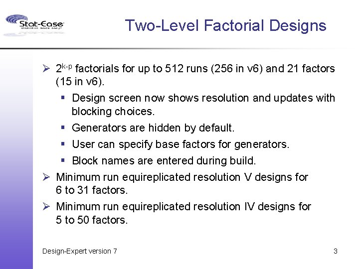
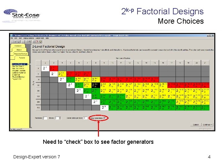
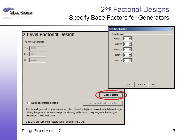
Two-Level Factorial Designs Ø 2 k-p factorials for up to 512 runs (256 in v 6) and 21 factors (15 in v 6). § Design screen now shows resolution and updates with blocking choices. § Generators are hidden by default. § User can specify base factors for generators. § Block names are entered during build. Ø Minimum run equireplicated resolution V designs for 6 to 31 factors. Ø Minimum run equireplicated resolution IV designs for 5 to 50 factors. Design-Expert version 7 3

2 k-p Factorial Designs More Choices Need to “check” box to see factor generators Design-Expert version 7 4

2 k-p Factorial Designs Specify Base Factors for Generators Design-Expert version 7 5

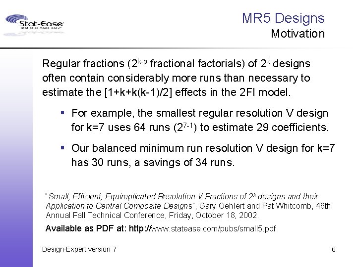
MR 5 Designs Motivation Regular fractions (2 k-p fractional factorials) of 2 k designs often contain considerably more runs than necessary to estimate the [1+k+k(k-1)/2] effects in the 2 FI model. § For example, the smallest regular resolution V design for k=7 uses 64 runs (27 -1) to estimate 29 coefficients. § Our balanced minimum run resolution V design for k=7 has 30 runs, a savings of 34 runs. “Small, Efficient, Equireplicated Resolution V Fractions of 2 k designs and their Application to Central Composite Designs”, Gary Oehlert and Pat Whitcomb, 46 th Annual Fall Technical Conference, Friday, October 18, 2002. Available as PDF at: http: //www. statease. com/pubs/small 5. pdf Design-Expert version 7 6

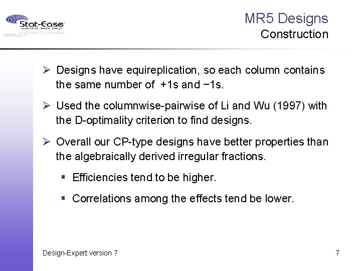
MR 5 Designs Construction Ø Designs have equireplication, so each column contains the same number of +1 s and − 1 s. Ø Used the columnwise-pairwise of Li and Wu (1997) with the D-optimality criterion to find designs. Ø Overall our CP-type designs have better properties than the algebraically derived irregular fractions. § Efficiencies tend to be higher. § Correlations among the effects tend be lower. Design-Expert version 7 7

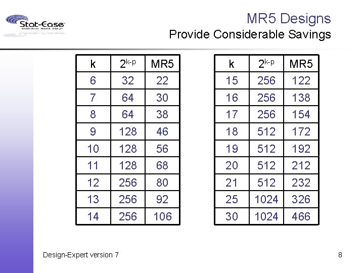
MR 5 Designs Provide Considerable Savings k 2 k-p MR 5 6 32 22 15 256 122 7 64 30 16 256 138 8 64 38 17 256 154 9 128 46 18 512 172 10 128 56 19 512 192 11 128 68 20 512 212 12 256 80 21 512 232 13 256 92 25 1024 326 14 256 106 30 1024 466 Design-Expert version 7 8

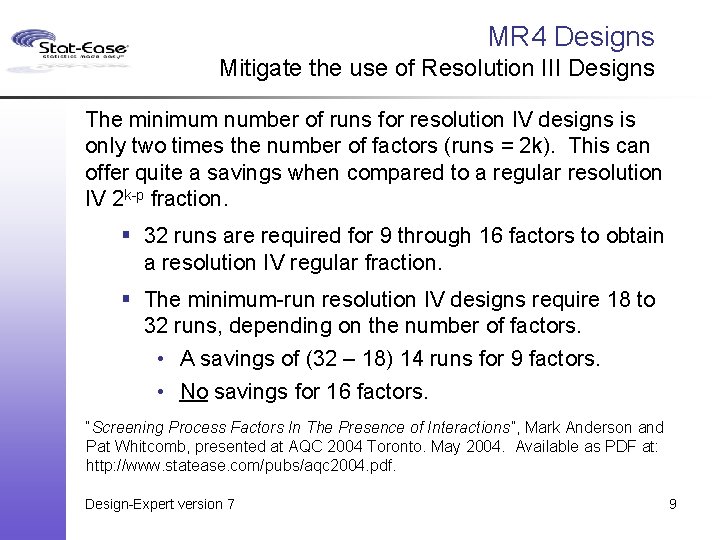
MR 4 Designs Mitigate the use of Resolution III Designs The minimum number of runs for resolution IV designs is only two times the number of factors (runs = 2 k). This can offer quite a savings when compared to a regular resolution IV 2 k-p fraction. § 32 runs are required for 9 through 16 factors to obtain a resolution IV regular fraction. § The minimum-run resolution IV designs require 18 to 32 runs, depending on the number of factors. • A savings of (32 – 18) 14 runs for 9 factors. • No savings for 16 factors. “Screening Process Factors In The Presence of Interactions”, Mark Anderson and Pat Whitcomb, presented at AQC 2004 Toronto. May 2004. Available as PDF at: http: //www. statease. com/pubs/aqc 2004. pdf. Design-Expert version 7 9

MR 4 Designs Suggest using “MR 4+2” Designs Problems: § If even 1 run lost, design becomes resolution III – main effects become badly aliased. § Reduction in runs causes power loss – may miss significant effects. Ø Evaluate power before doing experiment. Solution: § To reduce chance of resolution loss and increase power, consider adding some padding: Ø New Whitcomb & Oehlert “MR 4+2” designs Design-Expert version 7 10

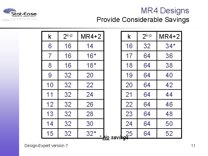
MR 4 Designs Provide Considerable Savings k 2 k-p MR 4+2 6 16 14 16 32 34* 7 16 16* 17 64 36 8 16 18* 18 64 38 9 32 20 19 64 40 10 32 22 20 64 42 11 32 24 21 64 44 12 32 26 22 64 46 13 32 28 23 64 48 14 32 30 24 64 50 15 32 32* 25 64 52 Design-Expert version 7 * No savings 11

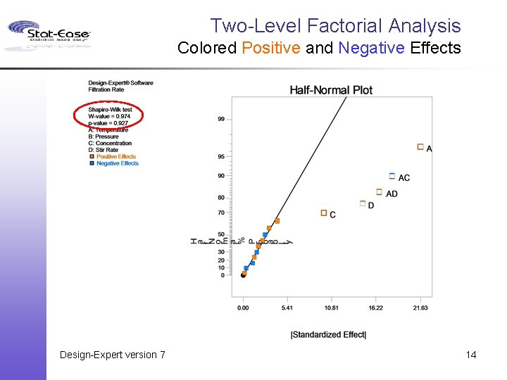
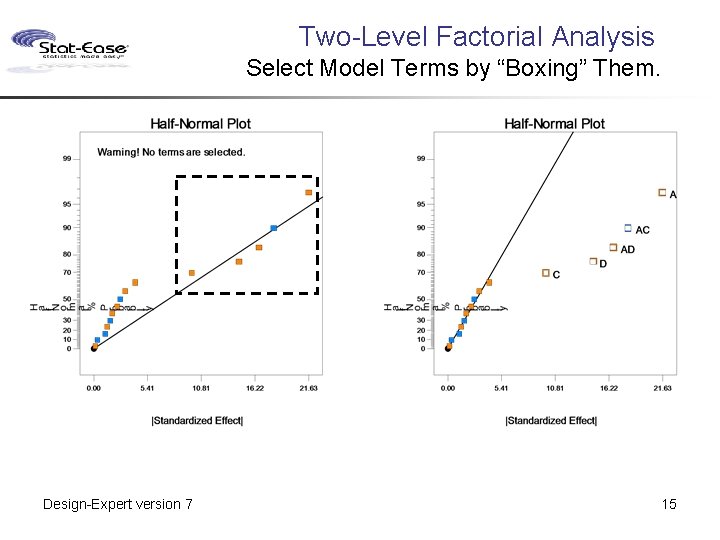
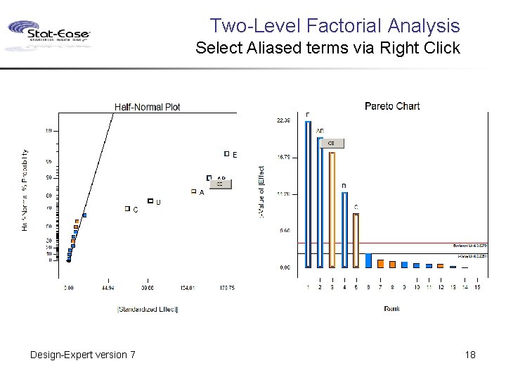
Two-Level Factorial Analysis Ø Effects Tool bar for model section tools. Ø Colored positive and negative effects and Shapiro-Wilk test statistic add to probability plots. Ø Select model terms by “boxing” them. Ø Pareto chart of t-effects. Ø Select aliased terms for model with right click. Ø Better initial estimates of effects in irregular factions by using “Design Model”. § Recalculate and clear buttons. Design-Expert version 7 12

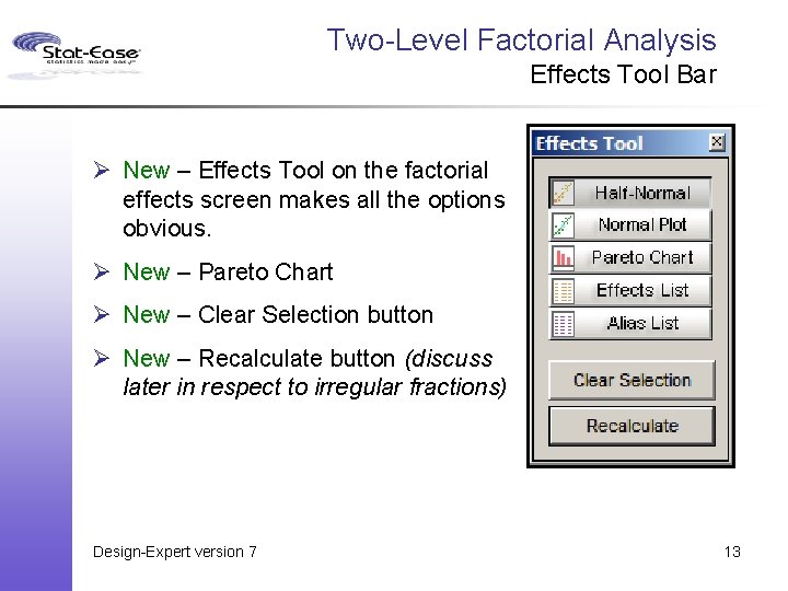
Two-Level Factorial Analysis Effects Tool Bar Ø New – Effects Tool on the factorial effects screen makes all the options obvious. Ø New – Pareto Chart Ø New – Clear Selection button Ø New – Recalculate button (discuss later in respect to irregular fractions) Design-Expert version 7 13

Two-Level Factorial Analysis Colored Positive and Negative Effects Design-Expert version 7 14

Two-Level Factorial Analysis Select Model Terms by “Boxing” Them. Design-Expert version 7 15

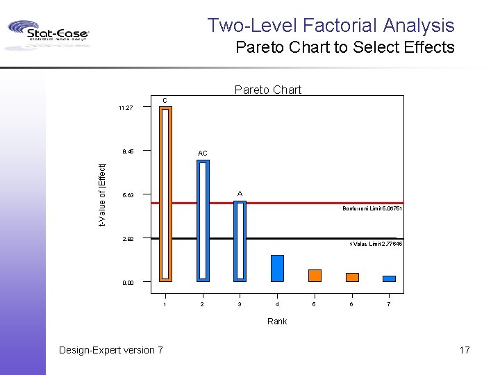
Two-Level Factorial Analysis Pareto Chart to Select Effects The Pareto chart is useful for showing the relative size of effects, especially to non-statisticians. Problem: If the 2 k-p factorial design is not orthogonal and balanced the effects have differing standard errors, so the size of an effect may not reflect its statistical significance. Solution: Plotting the t-values of the effects addresses the standard error problems for non-orthogonal and/or unbalanced designs. Problem: The largest effects always look large, but what is statistically significant? Solution: Put the t-value and the Bonferroni corrected t -value on the Pareto chart as guidelines. Design-Expert version 7 16

Two-Level Factorial Analysis Pareto Chart to Select Effects Pareto Chart C 11. 27 t-Value of |Effect| 8. 45 AC A 5. 63 Bonferroni Limit 5. 06751 2. 82 t-Value Limit 2. 77645 0. 00 1 2 3 4 5 6 7 Rank Design-Expert version 7 17

Two-Level Factorial Analysis Select Aliased terms via Right Click Design-Expert version 7 18

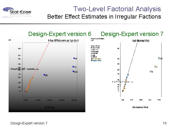
Two-Level Factorial Analysis Better Effect Estimates in Irregular Factions Design-Expert version 6 Design-Expert version 7 19

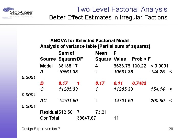
Two-Level Factorial Analysis Better Effect Estimates in Irregular Factions ANOVA for Selected Factorial Model Analysis of variance table [Partial sum of squares] Sum of Mean F Source Squares. DF Square Value Prob > F Model 38135. 17 4 9533. 79 130. 22 < 0. 0001 A 10561. 33 144. 25 < 0. 0001 B C 8. 17 1 11285. 33 8. 17 1 0. 11 0. 7482 11285. 33 154. 14 < AC 14701. 50 1 14701. 50 0. 0001 200. 80 < 0. 0001 Residual 512. 50 7 73. 21 Cor Total 38647. 67 Design-Expert version 7 11 20

Two-Level Factorial Analysis Better Effect Estimates in Irregular Factions Main effects only model: [Intercept] = Intercept - 0. 333*CD - 0. 333*ABC - 0. 333*ABD [A] = A - 0. 333*BC - 0. 333*BD - 0. 333*ACD [B] = B - 0. 333*AC - 0. 333*AD - 0. 333*BCD [C] = C - 0. 5*AB [D] = D - 0. 5*AB Main effects & 2 fi model: [Intercept] = Intercept - 0. 5*ABC - 0. 5*ABD [A] = A - ACD [B] = B - BCD [C] = C [D] = D [AB] = AB [AC] = AC - BCD [AD] = AD - BCD [BC] = BC - ACD [BD] = BD - ACD [CD] = CD - 0. 5*ABC - 0. 5*ABD Design-Expert version 7 21

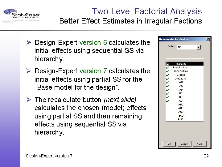
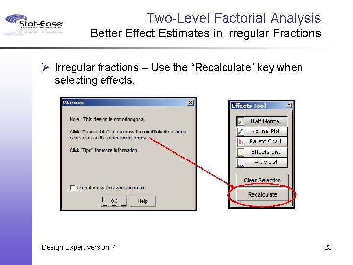
Two-Level Factorial Analysis Better Effect Estimates in Irregular Factions Ø Design-Expert version 6 calculates the initial effects using sequential SS via hierarchy. Ø Design-Expert version 7 calculates the initial effects using partial SS for the “Base model for the design”. Ø The recalculate button (next slide) calculates the chosen (model) effects using partial SS and then remaining effects using sequential SS via hierarchy. Design-Expert version 7 22

Two-Level Factorial Analysis Better Effect Estimates in Irregular Fractions Ø Irregular fractions – Use the “Recalculate” key when selecting effects. Design-Expert version 7 23

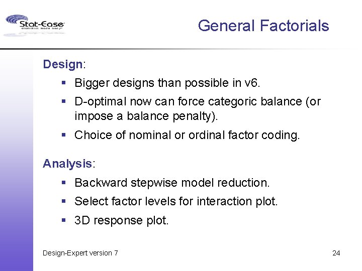
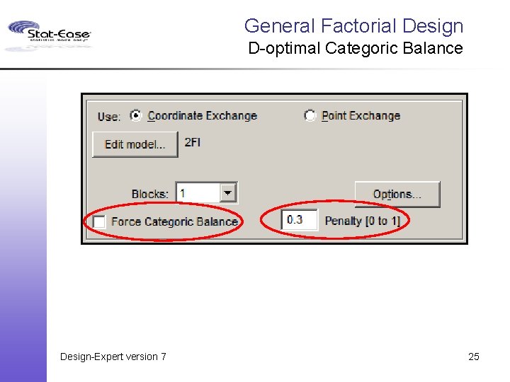
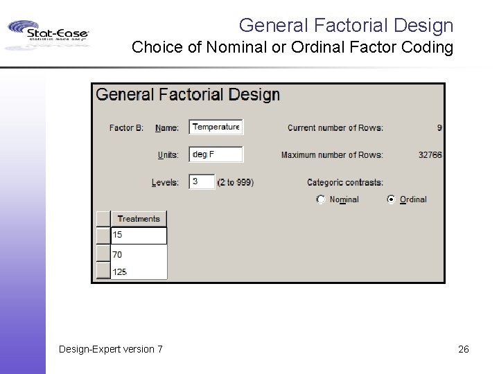
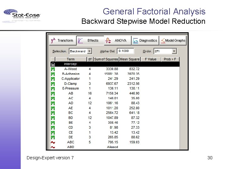
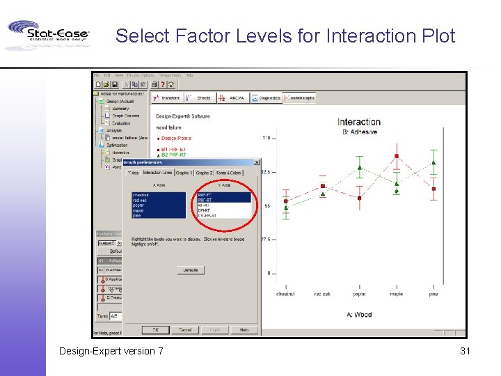
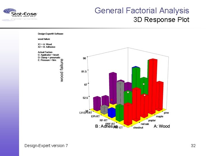
General Factorials Design: § Bigger designs than possible in v 6. § D-optimal now can force categoric balance (or impose a balance penalty). § Choice of nominal or ordinal factor coding. Analysis: § Backward stepwise model reduction. § Select factor levels for interaction plot. § 3 D response plot. Design-Expert version 7 24

General Factorial Design D-optimal Categoric Balance Design-Expert version 7 25

General Factorial Design Choice of Nominal or Ordinal Factor Coding Design-Expert version 7 26

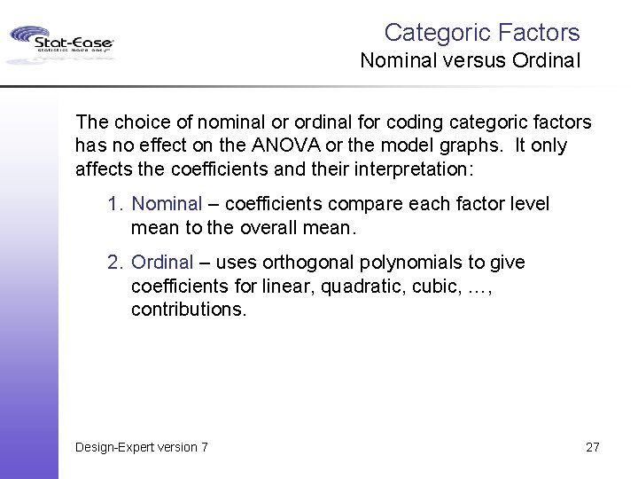
Categoric Factors Nominal versus Ordinal The choice of nominal or ordinal for coding categoric factors has no effect on the ANOVA or the model graphs. It only affects the coefficients and their interpretation: 1. Nominal – coefficients compare each factor level mean to the overall mean. 2. Ordinal – uses orthogonal polynomials to give coefficients for linear, quadratic, cubic, …, contributions. Design-Expert version 7 27

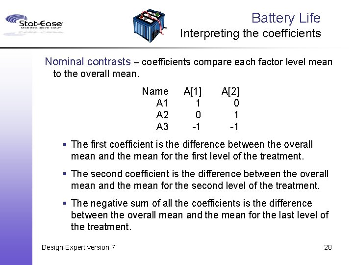
Battery Life Interpreting the coefficients Nominal contrasts – coefficients compare each factor level mean to the overall mean. Name A 1 A 2 A 3 A[1] 1 0 -1 A[2] 0 1 -1 § The first coefficient is the difference between the overall mean and the mean for the first level of the treatment. § The second coefficient is the difference between the overall mean and the mean for the second level of the treatment. § The negative sum of all the coefficients is the difference between the overall mean and the mean for the last level of the treatment. Design-Expert version 7 28

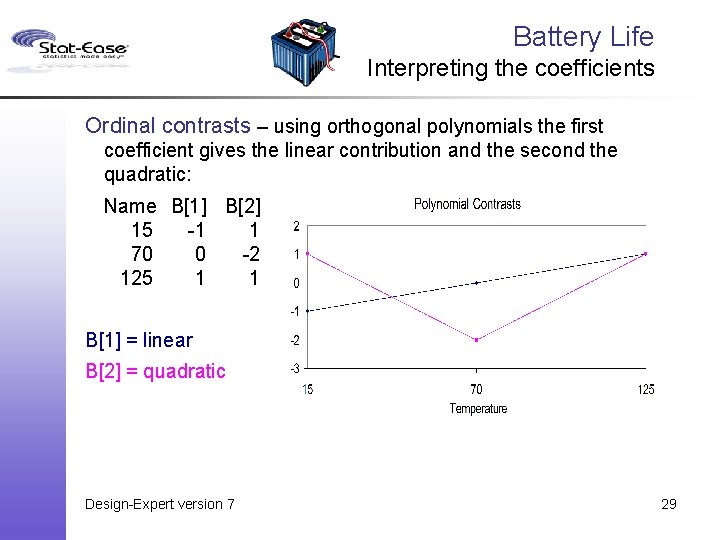
Battery Life Interpreting the coefficients Ordinal contrasts – using orthogonal polynomials the first coefficient gives the linear contribution and the second the quadratic: Name B[1] B[2] 15 -1 1 70 0 -2 125 1 1 B[1] = linear B[2] = quadratic Design-Expert version 7 29

General Factorial Analysis Backward Stepwise Model Reduction Design-Expert version 7 30

Select Factor Levels for Interaction Plot Design-Expert version 7 31

General Factorial Analysis 3 D Response Plot Design-Expert version 7 32

Factorial Design Augmentation Ø Semifold: Use to augment 2 k-p resolution IV; usually as many additional two-factor interactions can be estimated with half the runs as required for a full foldover. Ø Add Center Points. Ø Replicate Design. Ø Add Blocks. Design-Expert version 7 33

What’s New Ø General improvements § Design evaluation § Diagnostics § Updated graphics § Better help § Miscellaneous Cool New Stuff Ø Factorial design and analysis Ø Response surface design Ø Mixture design and analysis Ø Combined design and analysis Design-Expert version 7 34

Response Surface Designs Ø More “canned” designs; more factors and choices. § CCDs for ≤ 30 factors (v 6 ≤ 10 factors) • New CCD designs based on MR 5 factorials. • New choices for alpha “practical”, “orthogonal quadratic” and “spherical”. § Box-Behnken for 3– 30 factors (v 6 3, 4, 5, 6, 7, 9 & 10) § “Odd” designs moved to “Miscellaneous”. Ø Improved D-optimal design. § for ≤ 30 factors (v 6 ≤ 10 factors) § Coordinate exchange Design-Expert version 7 35

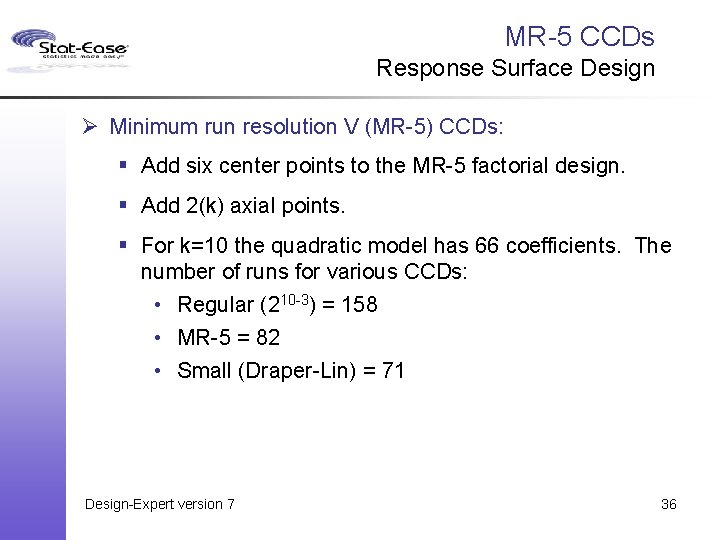
MR-5 CCDs Response Surface Design Ø Minimum run resolution V (MR-5) CCDs: § Add six center points to the MR-5 factorial design. § Add 2(k) axial points. § For k=10 the quadratic model has 66 coefficients. The number of runs for various CCDs: • Regular (210 -3) = 158 • MR-5 = 82 • Small (Draper-Lin) = 71 Design-Expert version 7 36

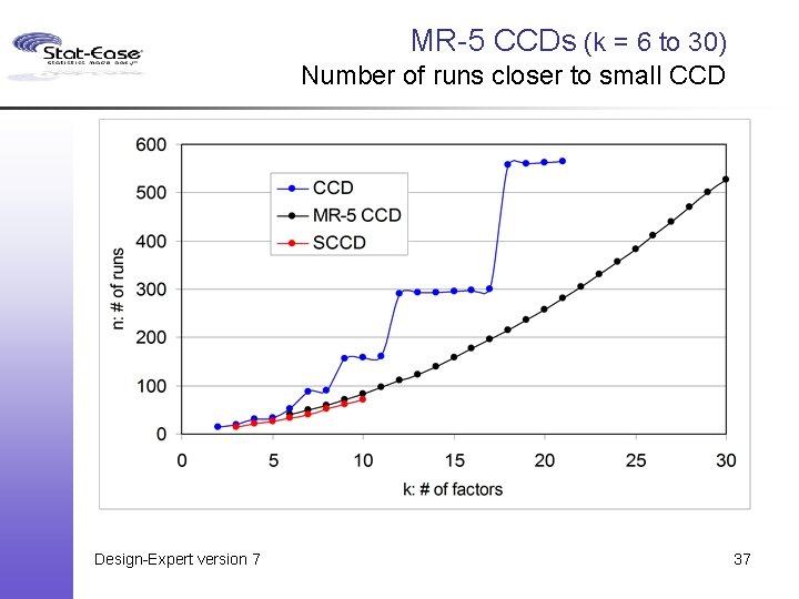
MR-5 CCDs (k = 6 to 30) Number of runs closer to small CCD Design-Expert version 7 37

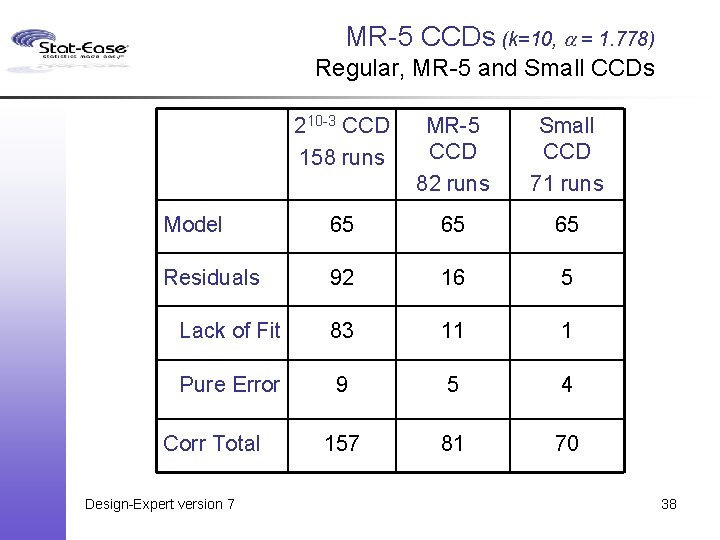
MR-5 CCDs (k=10, a = 1. 778) Regular, MR-5 and Small CCDs 210 -3 CCD 158 runs MR-5 CCD 82 runs Small CCD 71 runs Model 65 65 65 Residuals 92 16 5 Lack of Fit 83 11 1 Pure Error 9 5 4 157 81 70 Corr Total Design-Expert version 7 38

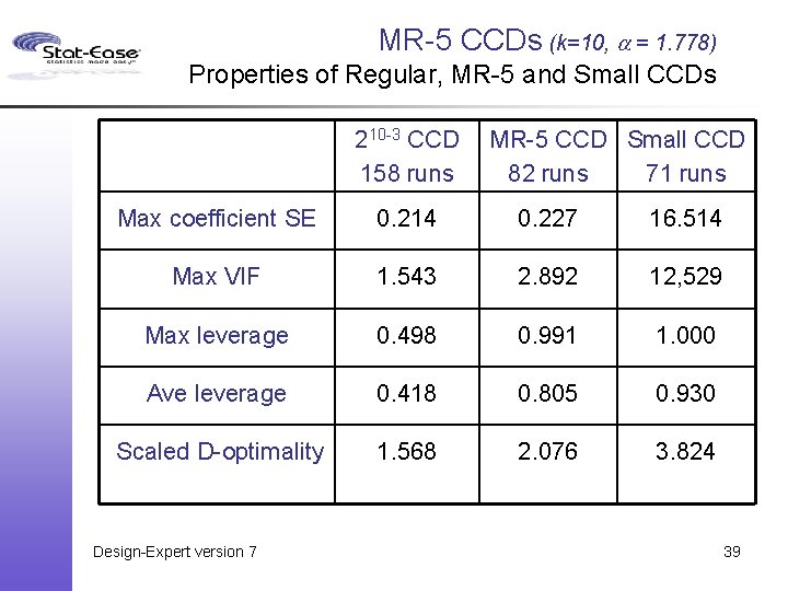
MR-5 CCDs (k=10, a = 1. 778) Properties of Regular, MR-5 and Small CCDs 210 -3 CCD 158 runs MR-5 CCD Small CCD 82 runs 71 runs Max coefficient SE 0. 214 0. 227 16. 514 Max VIF 1. 543 2. 892 12, 529 Max leverage 0. 498 0. 991 1. 000 Ave leverage 0. 418 0. 805 0. 930 Scaled D-optimality 1. 568 2. 076 3. 824 Design-Expert version 7 39

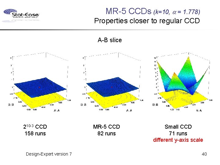
MR-5 CCDs (k=10, a = 1. 778) Properties closer to regular CCD A-B slice 210 -3 CCD 158 runs Design-Expert version 7 MR-5 CCD 82 runs Small CCD 71 runs different y-axis scale 40

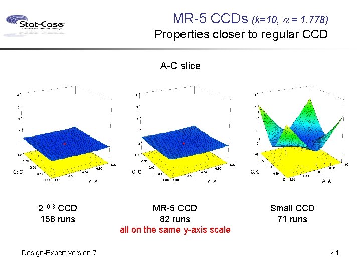
MR-5 CCDs (k=10, a = 1. 778) Properties closer to regular CCD A-C slice 210 -3 CCD 158 runs Design-Expert version 7 MR-5 CCD 82 runs all on the same y-axis scale Small CCD 71 runs 41

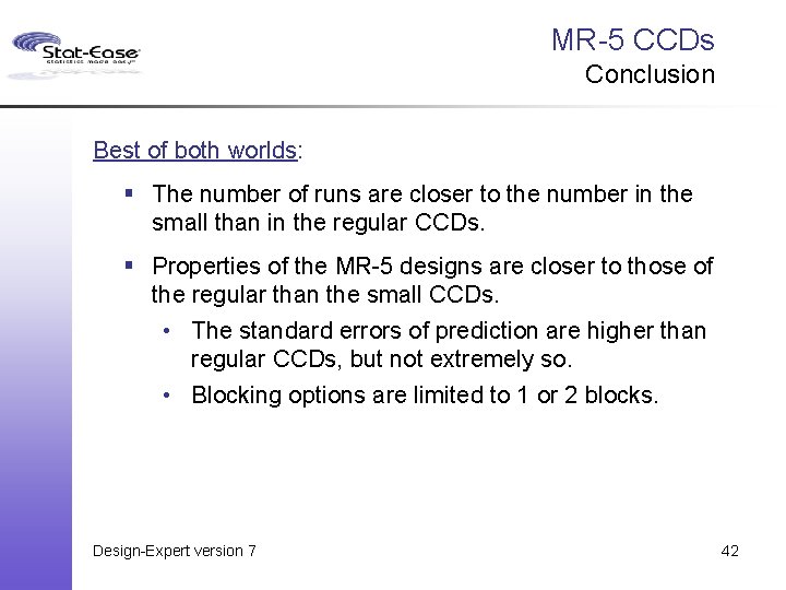
MR-5 CCDs Conclusion Best of both worlds: § The number of runs are closer to the number in the small than in the regular CCDs. § Properties of the MR-5 designs are closer to those of the regular than the small CCDs. • The standard errors of prediction are higher than regular CCDs, but not extremely so. • Blocking options are limited to 1 or 2 blocks. Design-Expert version 7 42

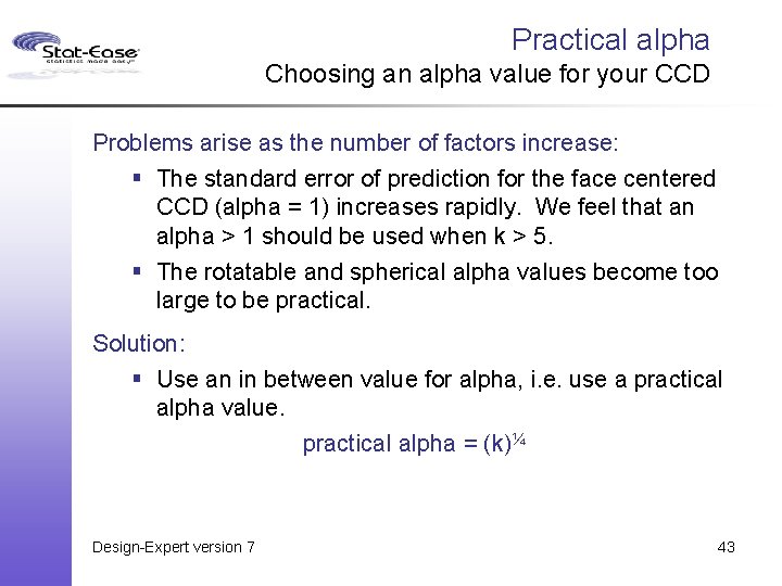
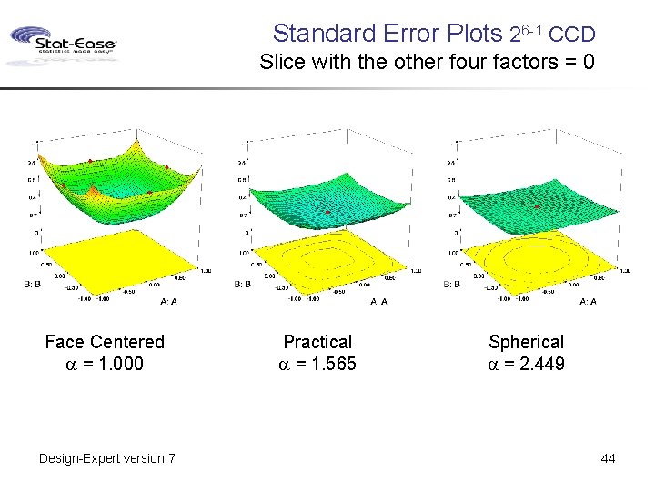
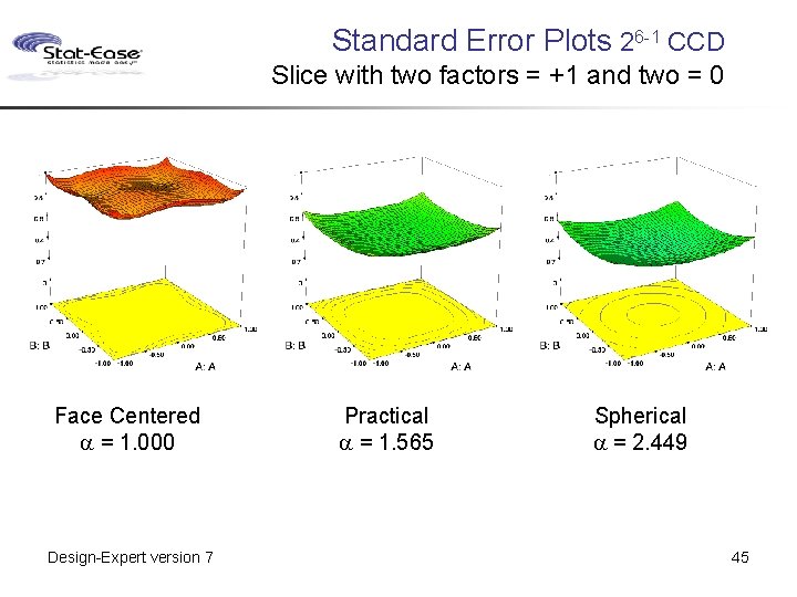
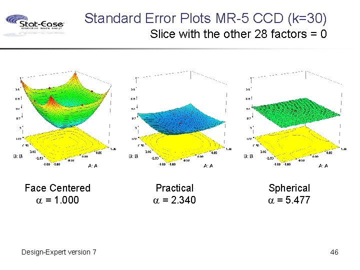
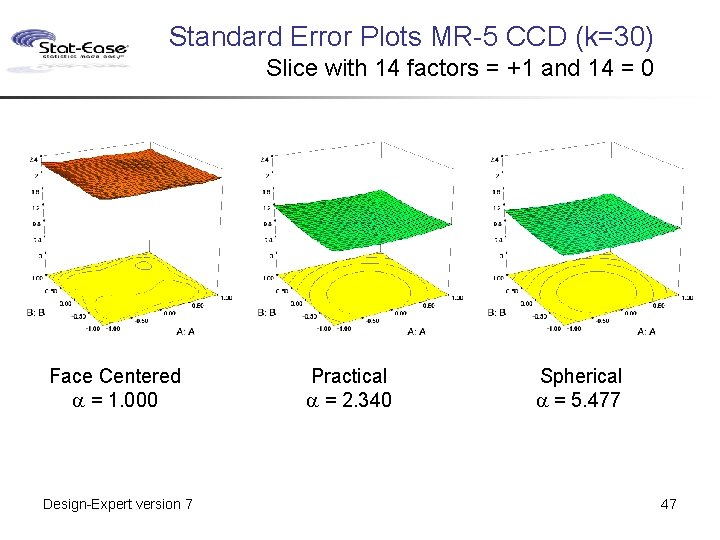
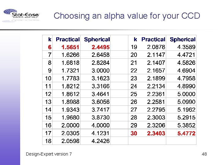
Practical alpha Choosing an alpha value for your CCD Problems arise as the number of factors increase: § The standard error of prediction for the face centered CCD (alpha = 1) increases rapidly. We feel that an alpha > 1 should be used when k > 5. § The rotatable and spherical alpha values become too large to be practical. Solution: § Use an in between value for alpha, i. e. use a practical alpha value. practical alpha = (k)¼ Design-Expert version 7 43

Standard Error Plots 26 -1 CCD Slice with the other four factors = 0 Face Centered a = 1. 000 Design-Expert version 7 Practical a = 1. 565 Spherical a = 2. 449 44

Standard Error Plots 26 -1 CCD Slice with two factors = +1 and two = 0 Face Centered a = 1. 000 Design-Expert version 7 Practical a = 1. 565 Spherical a = 2. 449 45

Standard Error Plots MR-5 CCD (k=30) Slice with the other 28 factors = 0 Face Centered a = 1. 000 Design-Expert version 7 Practical a = 2. 340 Spherical a = 5. 477 46

Standard Error Plots MR-5 CCD (k=30) Slice with 14 factors = +1 and 14 = 0 Face Centered a = 1. 000 Design-Expert version 7 Practical a = 2. 340 Spherical a = 5. 477 47

Choosing an alpha value for your CCD Design-Expert version 7 48

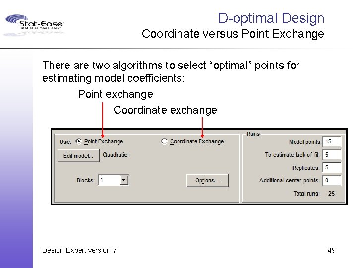
D-optimal Design Coordinate versus Point Exchange There are two algorithms to select “optimal” points for estimating model coefficients: Point exchange Coordinate exchange Design-Expert version 7 49

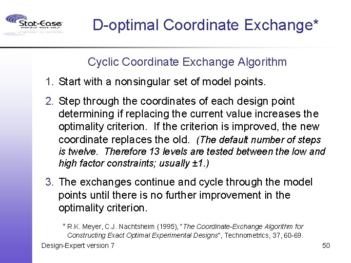
D-optimal Coordinate Exchange* Cyclic Coordinate Exchange Algorithm 1. Start with a nonsingular set of model points. 2. Step through the coordinates of each design point determining if replacing the current value increases the optimality criterion. If the criterion is improved, the new coordinate replaces the old. (The default number of steps is twelve. Therefore 13 levels are tested between the low and high factor constraints; usually ± 1. ) 3. The exchanges continue and cycle through the model points until there is no further improvement in the optimality criterion. * R. K. Meyer, C. J. Nachtsheim (1995), “The Coordinate-Exchange Algorithm for Constructing Exact Optimal Experimental Designs”, Technometrics, 37, 60 -69. Design-Expert version 7 50