NonExperimental designs Developmental designs SmallN designs Psych 231

Non-Experimental designs: Developmental designs & Small-N designs Psych 231: Research Methods in Psychology

Announcements Journal Summary 2 due this week n Bring your group project data to labs this week n – Decide how to analyze it • What test • Organize the data – Somebody from each group is encouraged to visit an office hour next week to finish the group project data analysis

Developmental designs n Used to study changes in behavior that occur as a function of age changes n Three major types – Cross-sectional • Age is subject variable treated as a between-subjects variable – Longitudinal – Cohort-sequential

Developmental designs n Longitudinal design – Follow the same individual or group over time • Age is treated as a within-subjects variable – – • Rather than comparing groups, the same individuals are compared to themselves at different times Repeated measurements over extended period of time Changes in dependent variable reflect changes due to aging process – Changes in performance are compared on an individual basis and overall

Developmental designs n Longitudinal design – Advantages: • Can see developmental changes clearly • Avoid some cohort effects (participants are all from same generation, so changes are more likely to be due to aging) • Can measure differences within individuals

Developmental designs n Longitudinal design – Disadvantages • Can be very time-consuming • Can have cross-generational effects: – Conclusions based on members of one generation may not apply to other generations • Numerous threats to internal validity: – Attrition/mortality – History – Practice effects » Improved performance over multiple tests may be due to practice taking the test • Cannot determine causality

Developmental designs n Cohort-sequential design – Measure groups of participants as they age • Example: measure a group of 5 year olds, then the same group 5 years later, as well as another group of 5 year olds – Age is both between and within subjects variable • Combines elements of cross-sectional and longitudinal designs • Addresses some of the concerns raised by other designs – For example, allows to evaluate the contribution of generation effects

Developmental designs n Cohort-sequential design – Advantages: • Can measure generation effect • Less time-consuming than longitudinal – Disadvantages: • Still time-consuming • Still cannot make causal claims

Small N designs n What are they? – Review Chapter 13 • One or a few participants • Data are not analyzed statistically; rather rely on visual interpretation of the data • Basic method – Observations begin in the absence of treatment (BASELINE) » Look for stable level – Then treatment is implemented – Changes in frequency, magnitude, or intensity of behavior are recorded

Statistics n Why do we use them? – Descriptive statistics • Used to describe, simplify, & organize data sets – Inferential statistics • Used to test claims about the population, based on data gathered from samples • Takes sampling error into account, are the results above and beyond what you’d expect by random chance

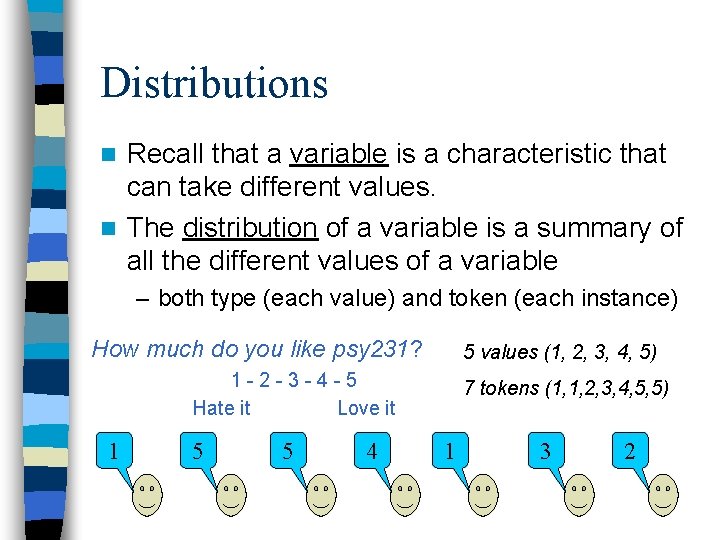
Distributions Recall that a variable is a characteristic that can take different values. n The distribution of a variable is a summary of all the different values of a variable n – both type (each value) and token (each instance) How much do you like psy 231? 5 values (1, 2, 3, 4, 5) 1 -2 -3 -4 -5 Hate it Love it 1 5 5 4 7 tokens (1, 1, 2, 3, 4, 5, 5) 1 3 2

Distribution Example: Distribution of scores on an exam – A frequency histogram Frequency n

Distributions n A picture of the distribution is usually helpful – Gives a good sense of the properties of the distribution n Many different ways to display distribution – Graphs • Continuous variable: – histogram, line graph (frequency polygons) • Categorical variable: – pie chart, bar chart – Table • Frequency distribution table • Stem and leaf plot

Graphs for continuous variables n Histogram n Line graph

Graphs for categorical variables n Bar chart n Pie chart

Frequency distribution table Values (types) Counts Percentages

Distribution n Properties of a distribution – Shape • Symmetric v. asymmetric (skew) • Unimodal v. multimodal – Center • Where most of the data in the distribution are – Mean, Median, Mode – Spread (variability) • How similar/dissimilar are the scores in the distribution? – Standard deviation (variance), Range

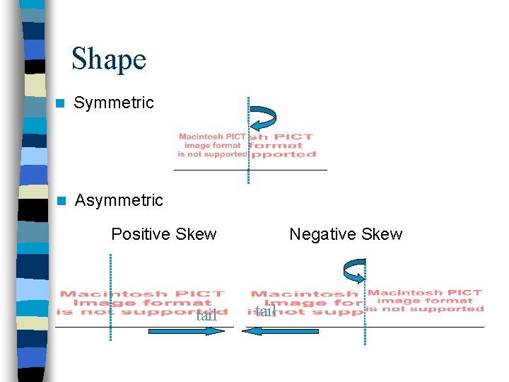
Shape n Symmetric n Asymmetric Positive Skew tail Negative Skew tail

Shape n n Unimodal (one mode) Multimodal – Bimodal examples Minor mode Major mode

Center n There are three main measures of center – Mean (M): the arithmetic average • Add up all of the scores and divide by the total number • Most used measure of center – Median (Mdn): the middle score in terms of location • The score that cuts off the top 50% of the from the bottom 50% • Good for skewed distributions (e. g. net worth) – Mode: the most frequent score • Good for nominal scales (e. g. eye color) • A must for multi-modal distributions

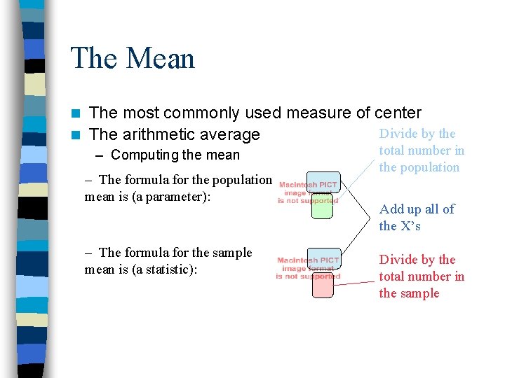
The Mean The most commonly used measure of center Divide by the n The arithmetic average n – Computing the mean – The formula for the population mean is (a parameter): – The formula for the sample mean is (a statistic): total number in the population Add up all of the X’s Divide by the total number in the sample

The Mean The most commonly used measure of center n The arithmetic average n – Computing the mean Our population 2, 4, 6, 8

Spread (Variability) n How similar are the scores? – Range: the maximum value - minimum value • Only takes two scores from the distribution into account • Influenced by extreme values (outliers) – Standard deviation (SD): (essentially) the average amount that the scores in the distribution deviate from the mean • Takes all of the scores into account • Also influenced by extreme values (but not as much as the range) – Variance: standard deviation squared

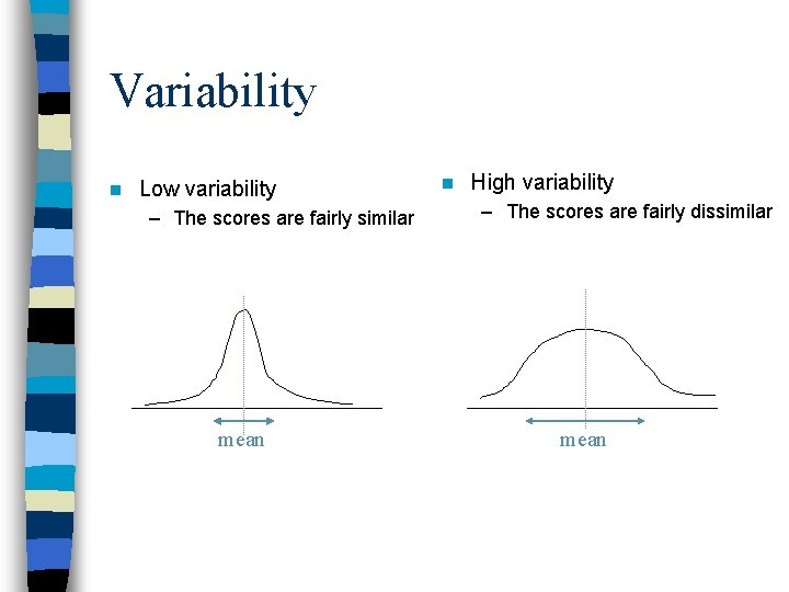
Variability n Low variability – The scores are fairly similar mean n High variability – The scores are fairly dissimilar mean

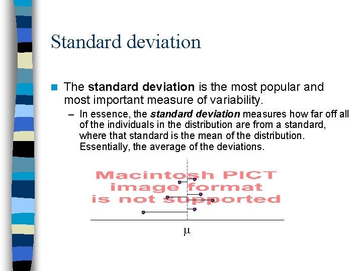
Standard deviation n The standard deviation is the most popular and most important measure of variability. – In essence, the standard deviation measures how far off all of the individuals in the distribution are from a standard, where that standard is the mean of the distribution. Essentially, the average of the deviations.

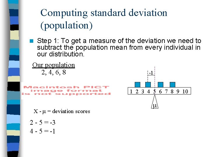
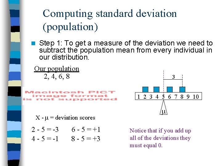
Computing standard deviation (population) n Step 1: To get a measure of the deviation we need to subtract the population mean from every individual in our distribution. Our population 2, 4, 6, 8 -3 1 2 3 4 5 6 7 8 9 10 X - = deviation scores 2 - 5 = -3

Computing standard deviation (population) n Step 1: To get a measure of the deviation we need to subtract the population mean from every individual in our distribution. Our population 2, 4, 6, 8 -1 1 2 3 4 5 6 7 8 9 10 X - = deviation scores 2 - 5 = -3 4 - 5 = -1

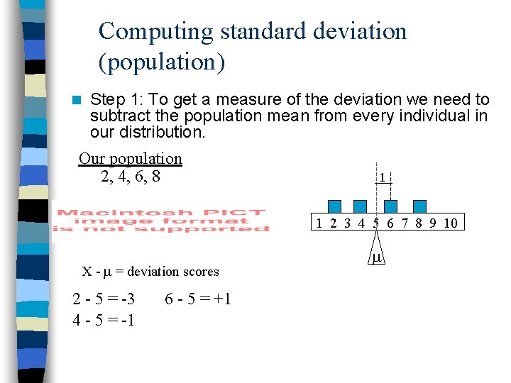
Computing standard deviation (population) n Step 1: To get a measure of the deviation we need to subtract the population mean from every individual in our distribution. Our population 2, 4, 6, 8 1 1 2 3 4 5 6 7 8 9 10 X - = deviation scores 2 - 5 = -3 4 - 5 = -1 6 - 5 = +1

Computing standard deviation (population) n Step 1: To get a measure of the deviation we need to subtract the population mean from every individual in our distribution. Our population 2, 4, 6, 8 3 1 2 3 4 5 6 7 8 9 10 X - = deviation scores 2 - 5 = -3 4 - 5 = -1 6 - 5 = +1 8 - 5 = +3 Notice that if you add up all of the deviations they must equal 0.

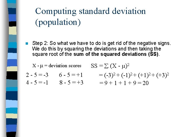
Computing standard deviation (population) n Step 2: So what we have to do is get rid of the negative signs. We do this by squaring the deviations and then taking the square root of the sum of the squared deviations (SS). X - = deviation scores 2 - 5 = -3 4 - 5 = -1 6 - 5 = +1 8 - 5 = +3 SS = (X - )2 = (-3)2 + (-1)2 + (+3)2 = 9 + 1 + 9 = 20

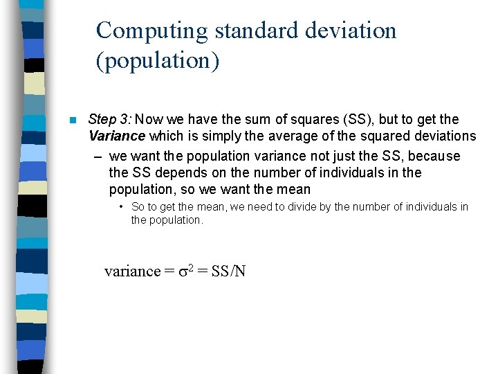
Computing standard deviation (population) n Step 3: Now we have the sum of squares (SS), but to get the Variance which is simply the average of the squared deviations – we want the population variance not just the SS, because the SS depends on the number of individuals in the population, so we want the mean • So to get the mean, we need to divide by the number of individuals in the population. variance = 2 = SS/N

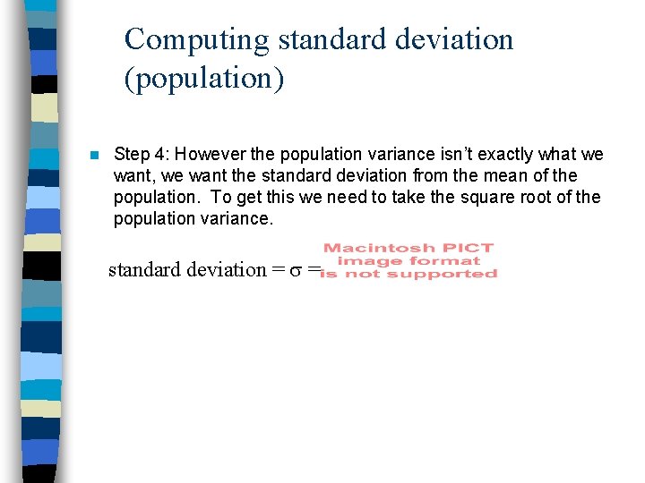
Computing standard deviation (population) n Step 4: However the population variance isn’t exactly what we want, we want the standard deviation from the mean of the population. To get this we need to take the square root of the population variance. standard deviation = =

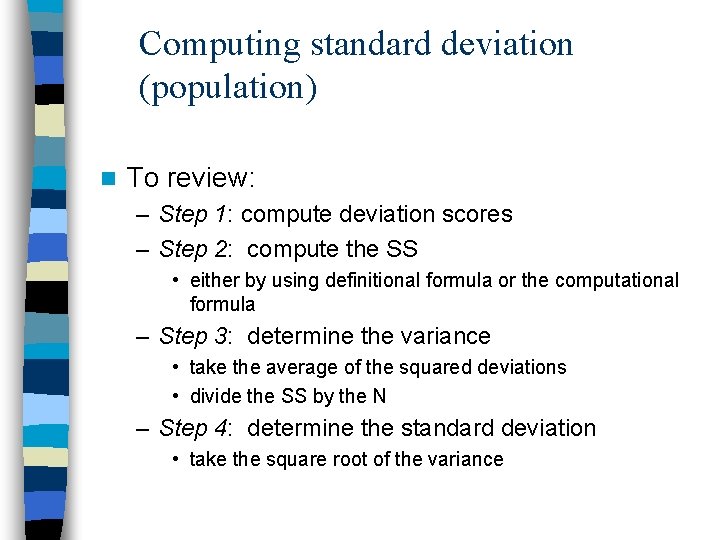
Computing standard deviation (population) n To review: – Step 1: compute deviation scores – Step 2: compute the SS • either by using definitional formula or the computational formula – Step 3: determine the variance • take the average of the squared deviations • divide the SS by the N – Step 4: determine the standard deviation • take the square root of the variance