Strategies for Information Extraction and Artifact Reduction in

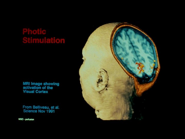
Strategies for Information Extraction and Artifact Reduction in Functional MRI Peter A. Bandettini, Ph. D Unit on Functional Imaging Methods & 3 T Neuroimaging Core Facility Laboratory of Brain and Cognition National Institute of Mental Health

Categories of Questions Asked with f. MRI Where? When? How much? --How to get the brain to do what we want it to do in the context of an f. MRI experiment? (limitations: limited time and signal to noise, motion, acoustic noise)

A Primary Challenge: . . . to make progressively more precise inferences using f. MRI without making too many assumptions about non-neuronal physiologic factors.

Neuronal Activation ? Measured f. MRI Signal Hemodynamics Physiologic Factors ?

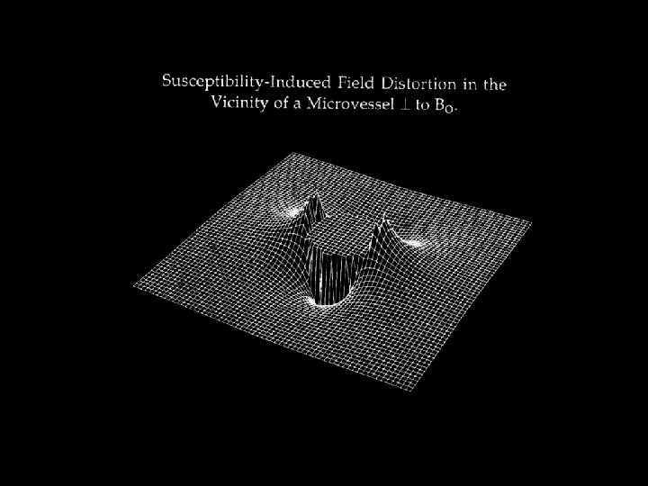
Physiologic Factors that Influence BOLD Contrast • • • Blood oxygenation Blood volume Blood pressure Hematocrit Vessel size Coupling: Flow & CMRO 2

Contrast in Functional MRI • Blood Volume – Contrast agent injection and time series collection of T 2* or T 2 - weighted images • BOLD – Time series collection of T 2* or T 2 - weighted images • Perfusion – T 1 weighting – Arterial spin labeling

Resting Active

BOLD Contrast in the Detection of Neuronal Activity Cerebral Tissue Activation Local Vasodilation Oxygen Delivery Exceeds Metabolic Need Increase in Cerebral Blood Flow and Volume Increase in Capillary and Venous Blood Oxygenation Deoxy-hemoglobin: paramagnetic diamagnetic Decrease in Deoxy-hemoglobin. Oxy-hemoglobin: Decrease in susceptibility-related intravoxel dephasing Increase in T 2 and T 2* Local Signal Increase in T 2 and T 2* - weighted sequences

The BOLD Signal Blood Oxygenation Level Dependent (BOLD) signal changes task

Perfusion / Flow Imaging EPISTAR - - - FAIR . . . Perfusion Time Series

TI (ms) 200 400 600 800 1000 1200 FAIR EPISTAR

Scanner and Hemodynamic Limits

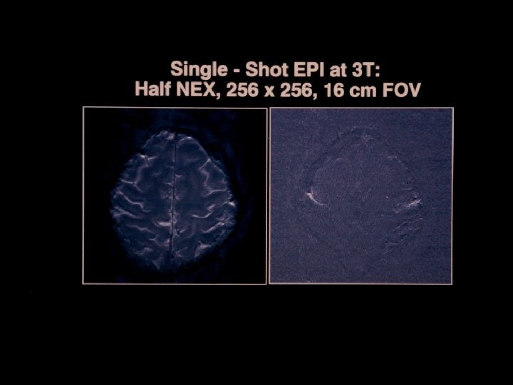
Single Shot Imaging T 2* decay EPI Readout Window ≈ 20 to 40 ms

Multishot Imaging T 2* decay EPI Window 1 T 2* decay EPI Window 2

Multi Shot EPI Excitations Matrix Size 1 64 x 64 2 128 x 128 4 256 x 128 8 256 x 256

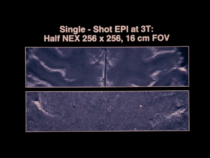
Partial k-space imaging T 2* decay EPI Window

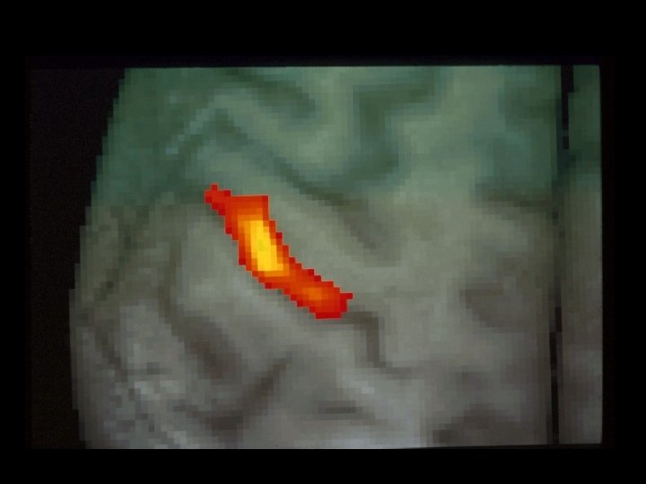
Perfusion BOLD Rest Activation

Anatomy BOLD Perfusion

Hemodynamic Specificity Arterial inflow (BOLD TR < 500 ms) Venous inflow (Perf. No VN)

+ Volume BOLD Perfusion - • unique information • baseline information • multislice trivial • invasive • low C / N for func. • highest C / N • easy to implement • multislice trivial • non invasive • highest temp. res. • complicated signal • no baseline info. • unique information • control over ves. size • baseline information • non invasive • multislice non trivial • lower temp. res. • low C / N

CMRO 2 -related BOLD signal deficit: CBF hypercapnia visual stimulation Hoge, et al. BOLD (% increase) 20 CBF (% increase) 15 10 5 0 -5 -10 0 200 400 600 800 1000 1200 1400 Time (seconds) 3 2 1 0 0 200 400 600 800 1000 1200 1400 Time (seconds) Simultaneous Perfusion and BOLD imaging during graded visual activation and hypercapnia N=12

Hoge, et al. CBF-CMRO 2 coupling 4 -10 +10 0 +20 CMRO 2 (% increase) BOLD (% increase) 25 3 2 1 20 15 10 5 0 0 0 10 20 30 40 Perfusion (% increase) 50 0 10 20 30 40 50 Perfusion (% increase) Characterizing Activation-induced CMRO 2 changes using calibration with hypercapnia

Hoge, et al. Computed CMRO 2 changes 40 30 20 10 0 -10 -20 -30 -40 Subject 1 Subject 2 %

f. MRI signal change dynamics. . .

2 1000 msec 100 msec 34 msec 1. 5 1 0. 5 0 -0. 5 -1 15 20 25 Time (sec) 30 35

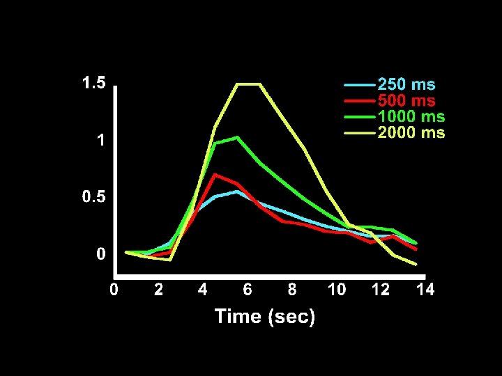
BOLD response is nonlinear Observed response Linear response 20 s 2000 ms 1000 ms 500 ms 250 ms 0 10 20 30 40 0 10 20 30 Short duration stimuli produce larger responses than expected 40

Source of the Nonlinearity • Neuronal • Hemodynamic – Miller et al. 1998 – Flow is linear, BOLD is nonlinear – Friston et al. 2000 – hemodynamics can explain nonlinearity If nonlinearity is hemodynamic in origin, a measure of this nonlinearity will reflect any spatial variation of the vasculature

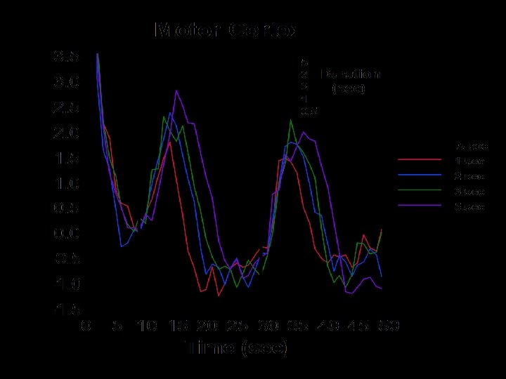
Methods Visual Motor … SD = 250 ms SD = 500 ms … SD = 500 ms SD = 1000 ms … SD = 1000 ms SD = 2000 ms … SD = 2000 ms SD = 4000 ms Stimulus Duration (SD) 16 s … 20 s Blocked Trial

Observed Responses measured ideal (linear) visual stimulation 250 ms 500 ms 1000 ms 2000 ms motor task 500 ms 1000 ms 2000 ms 4000 ms

Compute nonlinearity (for each voxel) • Amplitude of Response Fit ideal (linear) to response a • Area under response / Stimulus Duration Output Area / Input Area t

Nonlinearity Visual Magnitude 6 Output / input 6 4 4 2 2 linear Area f (SD) 0 1 2 3 4 Stimulus Duration 5 0 1 2 3 4 5 Stimulus Duration 6 Output / input f (SD) Motor 4 2 5 4 3 2 1 0 1 2 3 4 Stimulus Duration 5

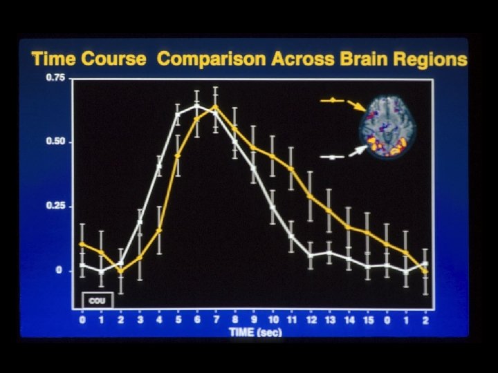
Results – visual task Nonlinearity Magnitude Latency

Results – motor task Nonlinearity Magnitude Latency

Results – visual task 8 f (SD) 6 4 2 0 1 -2 f (SD) 6 40 4 20 2 4 nonlinearity 6 3 4 5 0 10 20 30 40 8 60 02 2 Stimulus Duration 0 8 -2 1 2 3 4 5 Stimulus Duration

Results – motor task f (SD) 8 6 4 2 0 1 2 3 4 5 0 10 20 30 40 Stimulus Duration f (SD) 8 6 60 4 40 2 20 02 0 0 2 4 nonlinearity 6 8 1 2 3 4 Stimulus Duration 5 0 10 20 30 40

Reproducibility Motor task Nonlinearity 1 Visual task Nonlinearity 2 Experiment 1 Experiment 2

Latency Magnitude + 2 sec - 2 sec

Regions of Interest Used for Hemi-Field Experiment Right Hemisphere Left Hemisphere

9. 0 seconds 15 seconds 500 msec 10 20 Time (seconds) 30

Hemi-field with 500 msec asynchrony Average of 6 runs Standard Deviations Shown 3. 2 2. 4 1. 6 Percent 0. 8 MR Signal Strength 0 -0. 8 -1. 6 -2. 4 0 10 Time (seconds) 20 30

500 ms Right Hemifield Left Hemifield + 2. 5 s 0 s - 2. 5 s - =

250 ms Right Hemifield Left Hemifield + 2. 5 s 0 s - 2. 5 s - =

What is “in” the data? Neuronal Activation 1. Task Related & Time Locked 2. Task Related & Not Time Locked 3. Not Task Related Hemodynamics Cardiac Pulsation Respiration Motion MRI Signal Changes

Motion Recognize? • Edge effects • Shorter signal change latencies • Unusually high signal changes • External measuring devices Correct? • Image registration algorithms • Orthogonalize to motion-related function (cardiac, respiration, movement) • Navigator echo for k-space alignment (for multishot techniques) • Re-do scan Bypass? • Paradigm timing strategies. . • Gating (with T 1 -correction) Suppress? • Flatten image contrast • Physical restraint • Averaging, smoothing

0. 25 Hz Breathing at 1. 5 T 26 ms 49 ms 0 Hz 0. 25 0. 5 Respiration map Power Spectra Image 3 ms

0. 68 Hz Cardiac rate at 3 T Power Spectra Image 3 ms 26 ms Cardiac map 49 ms 0 Hz 0. 68 (aliased) 0. 5

Temporal vs. Spatial SNR- 3 T 49 ms 26 ms 49 ms 27 ms 50 ms SPIRAL 26 ms EPI

Another artifact. . . Auditory Activation by the Scanner. . .

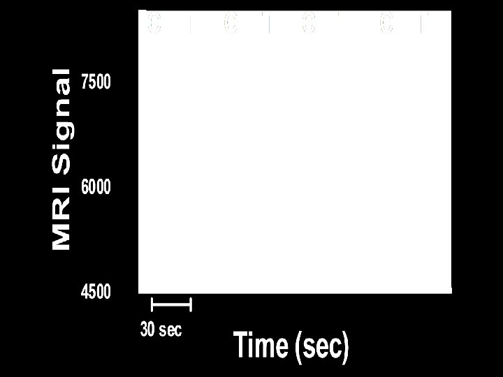
Prior EPI Gradients ( 20 sec ) Image Acquisition ( 20 to 30 sec) T C T T C = C Average Time Series Difference Time Series

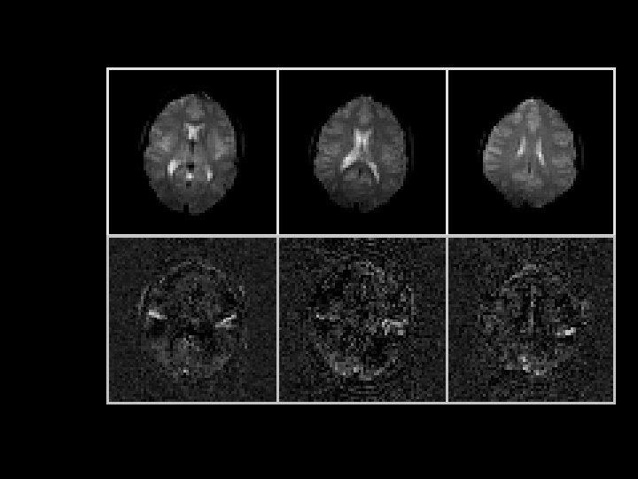
a. b. c. 0 1 2 3 4 Time (sec) 5 6 7

a.

b.

How to deal with Scanner Noise? • Clustered volume acquisition Talavage et al. • Silent sequences

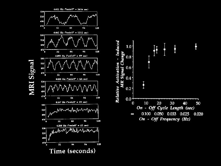
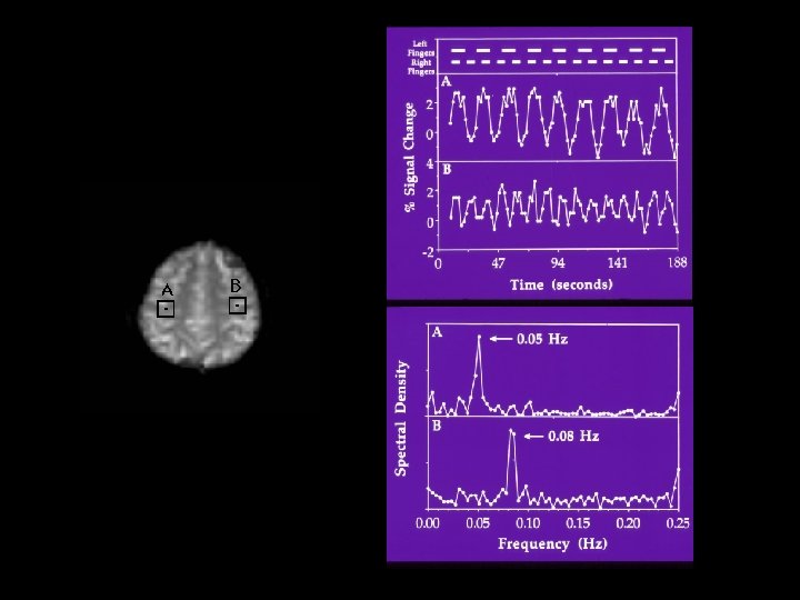
Neuronal Activation Input Strategies 1. Block Design 2. Frequency Encoding 3. Phase Encoding 4. Single Event 5. Orthogonal Block Design 6. Free behavior Design.

De. Yoe et al.

Neuronal Activation Input Strategies 1. Block Design 2. Frequency Encoding 3. Phase Encoding 4. Single Event 5. Orthogonal Block Design 6. Free behavior Design.

0. 08 Hz spectral density c. c. > 0. 5 with spectra 0. 05 Hz

Neuronal Activation Input Strategies 1. Block Design 2. Frequency Encoding 3. Phase Encoding 4. Single Event 5. Orthogonal Block Design 6. Free behavior Design.

Neuronal Activation Input Strategies 1. Block Design 2. Frequency Encoding 3. Phase Encoding 4. Single Event 5. Orthogonal Block Design 6. Free behavior Design.

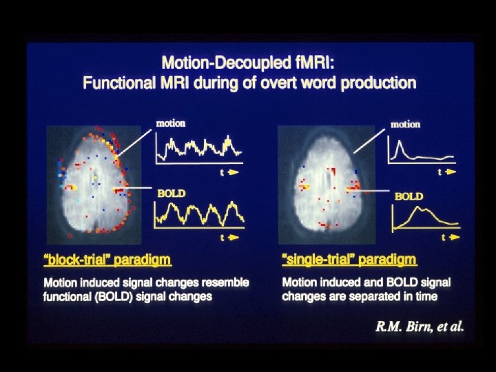
Overt Word Production 2 3 4 5 6 7 8 9 10 11 12 13

Tongue Movement Jaw Clenching

Neuronal Activation Input Strategies 1. Block Design 2. Frequency Encoding 3. Phase Encoding 4. Single Event 5. Orthogonal Block Design 6. Free behavior Design.

Example of a Set of Orthogonal Contrasts for Multiple Regression

Neuronal Activation Input Strategies 1. Block Design 2. Frequency Encoding 3. Phase Encoding 4. Single Event 5. Orthogonal Block Design 6. Free behavior Design.

Free Behavior Design Use a continuous measure as a reference function: • Task performance • Skin Conductance • Heart, respiration rate. . • Eye position • EEG

The Skin Conductance Response (SCR) Ventromedial PFC Orbitofrontal Cortex Hypothalamus Amygdala Sympathetic Nervous System Sweat Gland Resistance change across two electrodes induced by changes in sweating.

Skin conductance data collection • Equipment: UFI Bio. Derm Model 2701 Skin Conductance Meter, Slic-8000 8 -channel A>D converter, Slic Software for Windows. • • Time from stim. to T 1/2 : ~6 to 10 s 4000 mv range 0. 1 S = to 500 m. V amplitude 0. 05 S threshold • 1 S = 1 mmhos • • level: 250 m. V 1 - 3 sec • • 1 - 3 sec 8 - 14 sec Boucsein, Wolfram (1992). Electrodermal Activity. Plenum Press, NY Venables, Peter, (1991). Autonomic Activity ANYAS 620: 191 -207.

Activity correlated with SCR changes

Brain activity correlated with SCR during “Rest”

Processing Stream with Real Time f. MRI Stimulus Pulse Sequence Response Subject Scanner Image Reconstruction Image Registration/ Motion Detection Compute & Display Neuropsychological Stuff Investigator! Time Series Analyses

Reasons for real time f. MRI • Make sure you have good data before subject leaves the scanner • Repeat bad imaging runs • Provide feedback to subject (e. g. , “stop nodding your head!”) • Most important when dealing with patient populations – when FMRI is used for pre-surgical planning – when patients in study are hard to come by

Further Reasons. . • Adjustment of stimulus level to reach a R desired response magnitude – ½ of peak response – mapping of voxel stimulus-response curves • Carrying out experiment until some statistically significant result has been reached – Must pay attention to statisticians for this! – e. g. , do tasks until language lateralization has been established S

Things to Look At (à la AFNI ) Control Panel Displaying EP images from time series Graphing voxel time series data

Multislice layouts FIM overlaid on SPGR, in Talairach coords

Estimated subject movement parameters

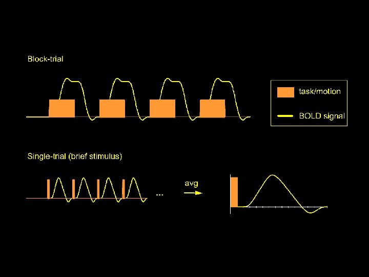
< 1 s to render Blocked trials: 20 s on/20 s off 8 blocks Blocks: 1 2345678 Color shows through brain Correlation > 0. 45 The End

Functional Imaging Methods / 3 T Group Staff Scientists: Sean Marrett Jerzy Bodurka Post Docs: Rasmus Birn Patrick Bellgowan Ziad Saad Clinical Fellow: James Patterson Graduate Student: Natalia Petridou Summer Students: Hannah Chang Courtney Kemps July 7, 2000