SizeDepth Tradeoff for Multiplying k Permutations Benjamin Rossman

Size-Depth Tradeoff for Multiplying k Permutations Benjamin Rossman Duke University
 : Given n-by-n permutation matrices M 1, …, Mk, compute (1, 1)-entry")
P(k, n) : Given n-by-n permutation matrices M 1, …, Mk, compute (1, 1)-entry of their product 0 1 2 ⋯ k– 1 k 1 1 2 3 ⋮ ⋮ n n
 : Given n-by-n permutation matrices M 1, …, Mk, compute (1, 1)-entry")
P(k, n) : Given n-by-n permutation matrices M 1, …, Mk, compute (1, 1)-entry of their product (M 1⋯Mk)1, 1 = 1 0 1 2 ⋯ k– 1 k 1 1 2 3 ⋮ ⋮ n n
 : Given n-by-n permutation matrices M 1, …, Mk, compute (1, 1)-entry")
P(k, n) : Given n-by-n permutation matrices M 1, …, Mk, compute (1, 1)-entry of their product (M 1⋯Mk)1, 1 = 0 0 1 2 ⋯ k– 1 k 1 1 2 3 ⋮ ⋮ n n
 : Given n-by-n permutation matrices M 1, …, Mk, compute (1, 1)-entry")
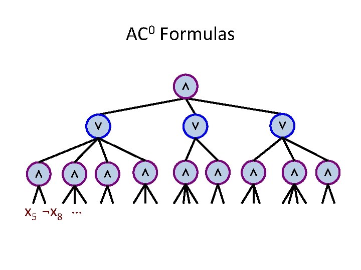
P(k, n) : Given n-by-n permutation matrices M 1, …, Mk, compute (1, 1)-entry of their product • This problem has depth d AC 0 formulas of size 1/d ) O(dk n ∧ ∨ ∧ ∧ ∨ ∨ ∧ ∧ ∧ ∧
 : Given n-by-n permutation matrices M 1, …, Mk, compute (1, 1)-entry")
P(k, n) : Given n-by-n permutation matrices M 1, …, Mk, compute (1, 1)-entry of their product AC 0 1/d ) O(dk n • This problem has depth d formulas of size • We give a nearly matching lower bound nΩ(dk 1/2 d ) (for small k), 1/exp(d)) improving previous nΩ(k bound [Beame, Impagliazzo, Pitassi’ 98]
 : Given n-by-n permutation matrices M 1, …, Mk, compute (1, 1)-entry")
P(k, n) : Given n-by-n permutation matrices M 1, …, Mk, compute (1, 1)-entry of their product 1/d ) O(dk n AC 0 • This problem has depth d formulas of size • We give a nearly matching lower bound nΩ(dk 1/2 d ) (for small k), 1/exp(d)) improving previous nΩ(k bound [Beame, Impagliazzo, Pitassi’ 98] • Obtained via “lifting” from a simpler complexity measure on join-trees for Pathk e 4 e 1 e 8 e 4 e 6 e 2 e 3 e 7 e 5 e 1 e 2 e 4 e 3 e 8 e 3 e 1 e 4 e 1 e 2 e 3 e 4 e 5 e 6 e 7 e 8

Plan 1. A combinatorial “toothpick” problem 2. Complexity of multiplying k permutations

a “toothpick” problem
")
rows of toothpicks (unit-length intervals)
![covering an interval of length k [0, k]](http://slidetodoc.com/presentation_image/210024eb906b639979b8cd212fbde9f9/image-11.jpg "covering an interval of length k [0, k]")
covering an interval of length k [0, k]

score = …

score = 3 + …

score = 3 + …

score = 3 + … “shadow” kills all toothpicks below it

score = 3 + …

score = 3 + 1 + …

score = 3 + 1 + …

score = 3 + 1 + 0 + …

score = 3 + 1 + 0 + …

score = 3 + 1 + 0 + …

score = 3 + 1 + 0 + …

score = 3 + 1 + 0 + 1 + …

score = 3 + 1 + 0 + 1 + …

score = 3 + 1 + 0 + …

score = 3 + 1 + 0 + 0

score = 3 + 1 + 0 + 0 = 5

score = 3 + 1 + 0 + 0 = 5

re-ordering rows

re-ordering rows

score: 6
")
a bad order (score 1)
")
a bad order (score 1)
")
a bad order (score 1)
")
a good re-ordering (score 5)
")
a good re-ordering (score 5)
")
a good re-ordering (score 5)
![Theorem For any covering of [0, k] by rows of “toothpicks” (unit-length intervals), there](http://slidetodoc.com/presentation_image/210024eb906b639979b8cd212fbde9f9/image-38.jpg "Theorem For any covering of [0, k] by rows of “toothpicks” (unit-length intervals), there")
Theorem For any covering of [0, k] by rows of “toothpicks” (unit-length intervals), there exists an ordering that achieves score ≥ k/6
![Theorem For any covering of [0, k] by rows of “toothpicks” (unit-length intervals), there](http://slidetodoc.com/presentation_image/210024eb906b639979b8cd212fbde9f9/image-39.jpg "Theorem For any covering of [0, k] by rows of “toothpicks” (unit-length intervals), there")
Theorem For any covering of [0, k] by rows of “toothpicks” (unit-length intervals), there exists an ordering that achieves score ≥ k/6 • Proof analyzes the obvious greedy algorithm: repeatedly select the next row that maximizes the gain in score


length: 41

length: 41 score: 10

max toothpicks in row: 3 length: 41 score: 10

max toothpicks in row: t length: 3 t 2 + 4 t + 2 score: (t+2)(t+1)/2

max toothpicks in row: t length: 3 t 2 + 4 t + 2 score: (t+2)(t+1)/2 Best possible ratio given t under the greedy algorithm!
 = (2 t choose")
Established using LP duality for a linear program with Catalan(t) = (2 t choose t) variables that bounds the performance of the greedy algorithm max toothpicks in row: t length: 3 t 2 + 4 t + 2 score: (t+2)(t+1)/2 Best possible ratio given t under the greedy algorithm!

intervals of different lengths

score: 4 + …

score: 4 + …

score: 4 + 2 + …

score: 4 + 2 + …

score: 4 + 2 + 1 + …

score: 4 + 2 + 1 + 0 + …

score: 4 + 2 + 1 + 0

score: 4 + 2 + 1 + 0 = 7

score: 4 + 2 + 1 + 0 = 7
![Theorem For any covering of [0, k] by rows of unit-length intervals, there exists](http://slidetodoc.com/presentation_image/210024eb906b639979b8cd212fbde9f9/image-57.jpg "Theorem For any covering of [0, k] by rows of unit-length intervals, there exists")
Theorem For any covering of [0, k] by rows of unit-length intervals, there exists an ordering that achieves score ≥ k/6
![Theorem For any covering of [0, k] by rows of intervals of length ≤](http://slidetodoc.com/presentation_image/210024eb906b639979b8cd212fbde9f9/image-58.jpg "Theorem For any covering of [0, k] by rows of intervals of length ≤")
Theorem For any covering of [0, k] by rows of intervals of length ≤ �� , there exists an ordering that achieves score ≥ k/6��
![Theorem For any covering of [0, k] by rows of intervals of length ≤](http://slidetodoc.com/presentation_image/210024eb906b639979b8cd212fbde9f9/image-59.jpg "Theorem For any covering of [0, k] by rows of intervals of length ≤")
Theorem For any covering of [0, k] by rows of intervals of length ≤ �� , there exists an ordering that achieves score ≥ k/6�� • This theorem underlies our size-depth tradeoff for SAC 0 formulas!
![Theorem For any covering of [0, k] by rows of intervals of length ≤](http://slidetodoc.com/presentation_image/210024eb906b639979b8cd212fbde9f9/image-60.jpg "Theorem For any covering of [0, k] by rows of intervals of length ≤")
Theorem For any covering of [0, k] by rows of intervals of length ≤ �� , there exists an ordering that achieves score ≥ k/6�� • [0, k] ☞ the graph Pathk 0 1 2 ⋯ • row of intervals ☞ subgraph of Pathk • “ordering” ☞ “permutation” k
 Theorem For any covering of Pathk by subgraphs G 1, …, Gm with")
(Same) Theorem For any covering of Pathk by subgraphs G 1, …, Gm with component length ≤ �� , there exists a permutation �� such that Score(G�� (1), …, G�� (m)) ≥ k/6�� • [0, k] ☞ the graph Pathk 0 1 2 ⋯ • row of intervals ☞ subgraph of Pathk • “ordering” ☞ “permutation” k
 Theorem For any covering of Pathk by subgraphs G 1, …, Gm with")
(Same) Theorem For any covering of Pathk by subgraphs G 1, …, Gm with component length ≤ �� , there exists a permutation �� such that Score(G�� (1), …, G�� (m)) ≥ k/6�� • We next restrict the class of allowed permutations ��

Shift Permutations • A shift permutation is a permutation �� on {1, …, m}, in which every cycle has the form i → i+1 → … → j– 1 → j • Example: �� = (1 2 3)(4)(5 6 7 8)(9 10) 1→ 2→ 3 4 ↻ 5→ 6→ 7→ 8 9 ↔� 10
(2 3)(4 5)(6 7)…")
another example: (1)(2 3)(4 5)(6 7)…

Theorem 1 For any covering of Pathk by subgraphs G 1, …, Gm with component length ≤ �� , there exists a permutation �� such that Score(G�� (1), …, G�� (m)) ≥ k/6�� Theorem 2 For any covering of Pathk by subgraphs G 1, …, Gm with component length ≤ �� , there exists a shift permutation �� s. t. Score(G�� (1), …, G�� (m)) ≥ k/10��

Theorem 1 For any covering of Pathk by subgraphs G 1, …, Gm with component length ≤ �� , there exists a permutation �� such that Score(G�� (1), …, G�� (m)) ≥ k/6�� Theorem 2 For any covering of Pathk by subgraphs G 1, …, Gm with component length ≤ �� , there exists a shift permutation �� s. t. Score(G�� (1), …, G�� (m)) ≥ k/10�� • Theorem 2 underlies our size-depth tradeoff for AC 0 formulas! • The bound Ω( k/�� ) is best possible
 is best score under shift permutations")
O( k) is best score under shift permutations
 is best score under shift permutations")
O( k) is best score under shift permutations
 is best score under shift permutations")
O( k) is best score under shift permutations

Plan 1. A combinatorial “toothpick” problem 2. Complexity of multiplying k permutations

De. Morgan Formulas ∧ ¬ ∨ ∨ ¬ ∧ ∧ x 4 ∨ x 2 x 3 x 1 ¬ x 2 ∧ ¬ ¬ x 3 ∧ ∧ x 4 ∨ x 4 x 5 x 1 x 5
 : Given n-by-n permutation matrices M 1, …, Mk, compute (1, 1)-entry")
P(k, n) : Given n-by-n permutation matrices M 1, …, Mk, compute (1, 1)-entry of their product (M 1⋯Mk)1, 1 = 1 0 1 2 ⋯ k– 1 k 1 1 2 3 ⋮ ⋮ n n
")
Complexity of P(k, n)
 • P(k, 2) is equivalent to PARITYk 0 1 2")
Complexity of P(k, n) • P(k, 2) is equivalent to PARITYk 0 1 2 ⋯ k– 1 k 1 1 2 2
 • P(k, 2) is equivalent to PARITYk 0 1 2")
Complexity of P(k, n) • P(k, 2) is equivalent to PARITYk 0 1 2 ⋯ k– 1 k 1 1 2 2
 • P(k, 2) is equivalent to PARITYk • P(k, 5)")
Complexity of P(k, n) • P(k, 2) is equivalent to PARITYk • P(k, 5) is complete for NC 1 (Barrington’s Theorem) ∧ ¬ NC 1 = { languages with poly-size De. Morgan formulas } ∨ ∨ ¬ ∧ ∧ x 4 ∨ x 2 x 3 x 1 ¬ x 2 ∧ ¬ ¬ x 3 ∧ ∧ x 4 ∨ x 4 x 5 x 1 x 5
 • P(k, 2) is equivalent to PARITYk • P(k, 5)")
Complexity of P(k, n) • P(k, 2) is equivalent to PARITYk • P(k, 5) is complete for NC 1 (Barrington’s Theorem) • P(n, n) is complete for Logspace
 • P(k, 2) is equivalent to PARITYk • P(k, 5)")
Complexity of P(k, n) • P(k, 2) is equivalent to PARITYk • P(k, 5) is complete for NC 1 (Barrington’s Theorem) • P(n, n) is complete for Logspace A super-polynomial formula size lower bound for P(k, n) (for any k, n �∞) would separate NC 1 and Logspace
")
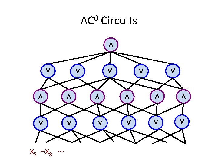
AC 0 Complexity of P(k, n)
 Computable by: § AC 0 formulas of size")
AC 0 Complexity of P(k, n) Computable by: § AC 0 formulas of size n. O(log k) and depth 2 log k
 Computable by: § AC 0 formulas of size")
AC 0 Complexity of P(k, n) Computable by: § AC 0 formulas of size n. O(log k) and depth 2 log k “recursive doubling”
 Computable by: § AC 0 formulas of size")
AC 0 Complexity of P(k, n) Computable by: § AC 0 formulas of size n. O(log k) and depth 2 log k § AC 0 formulas of size n. O(dk 1/d ) and depth 2 d ≤ 2 log k
 Computable by: § AC 0 formulas of size")
AC 0 Complexity of P(k, n) Computable by: § AC 0 formulas of size n. O(log k) and depth 2 log k § AC 0 formulas of size n. O(dk 1/d ) and depth 2 d ≤ 2 log k where �� : = k(d– 1)/d
 Computable by: § AC 0 formulas of size")
AC 0 Complexity of P(k, n) Computable by: § AC 0 formulas of size n. O(log k) and depth 2 log k § AC 0 formulas of size n. O(dk 1/d ) and depth 2 d ≤ 2 log k where �� : = k(d– 1)/d 2(d– 1) formula for P(�� Σ 2 d formula for P(k, n) = ORn�� /k ∘ AND , n) �� /k ∘ Σ
 Computable by: § AC 0 formulas of size")
AC 0 Complexity of P(k, n) Computable by: § AC 0 formulas of size n. O(log k) and depth 2 log k § AC 0 formulas of size n. O(dk 1/d ) and depth 2 d ≤ 2 log k
 Computable by: § AC 0 formulas of size")
AC 0 Complexity of P(k, n) Computable by: § AC 0 formulas of size n. O(log k) and depth log k § AC 0 formulas of size n. O(dk 1/d ) and depth d+1 ≤ log k
 Computable by: § AC 0 formulas of size")
AC 0 Complexity of P(k, n) Computable by: § AC 0 formulas of size n. O(log k) and depth log k § AC 0 formulas of size n. O(dk 1/d ) and depth d+1 ≤ log k P(k, n) has both DNF and CNF formulas of size O(nk):
 Computable by: § AC 0 formulas of size")
AC 0 Complexity of P(k, n) Computable by: § AC 0 formulas of size n. O(log k) and depth log k § AC 0 formulas of size n. O(dk 1/d ) and depth d+1 ≤ log k [Hastad‘ 86, R. ‘ 15] 1/d § Tight 2Ω(dk ) tradeoff when n = 2 (i. e. , for Parityk)
 Computable by: § AC 0 formulas of size")
AC 0 Complexity of P(k, n) Computable by: § AC 0 formulas of size n. O(log k) and depth log k § AC 0 formulas of size n. O(dk 1/d ) and depth d+1 ≤ log k [Hastad‘ 86, R. ‘ 15] 1/d § Tight 2Ω(dk ) tradeoff when n = 2 (i. e. , for Parityk) [Beame-Impagliazzo-Pitassi ‘ 98] 1/exp(d)) § nΩ(k tradeoff for AC 0 circuits computing P(k, n) (k ≤ log n)
 Computable by: § AC 0 formulas of size")
AC 0 Complexity of P(k, n) Computable by: § AC 0 formulas of size n. O(log k) and depth log k § AC 0 formulas of size n. O(dk 1/d ) and depth d+1 ≤ log k [Hastad‘ 86, R. ‘ 15] 1/d § Tight 2Ω(dk ) tradeoff when n = 2 (i. e. , for Parityk) [Beame-Impagliazzo-Pitassi ‘ 98] 1/exp(d)) § nΩ(k tradeoff for AC 0 circuits computing P(k, n) (k ≤ log n) [Chen-Oliveira-Servedio-Tan ‘ 16] 1/d § nΩ(k ) tradeoff for AC 0 circuits computing k-STCONN (k ≤ n 1/5) (via reduction to a problem with linear formula size)
 Computable by: § AC 0 formulas of size")
AC 0 Complexity of P(k, n) Computable by: § AC 0 formulas of size n. O(log k) and depth log k § AC 0 formulas of size n. O(dk 1/d ) and depth d+1 ≤ log k Our results: (k ≤ log n) § [R. ’ 14] Tight nΩ(log k) lower bound up to depth O~(log n) § [new] Nearly tight nΩ(dk 1/2 d) tradeoff for depth d+1 ≤ log k
 join-trees for Pathk (the path")
The Pathset Framework AC 0 formulas solving P(k, n) join-trees for Pathk (the path graph of length k)

The Pathset Framework This reduction lets us “lift” lower bounds for join-trees to lower bounds for AC 0 formulas [R. ’ 14] (as well as unbounded-depth monotone formulas [R. ’ 15]) AC 0 formulas solving P(k, n) join-trees for Pathk (the path graph of length k)

The Pathset Framework equivalent De. Morgan formulas pathset formulas AC 0 formulas solving P(k, n) join-trees for Pathk (fan-in 2, logarithmic depth) (the path graph of length k)
 pathset formulas Circuit")
The Pathset Framework equivalent De. Morgan formulas (fan-in 2, logarithmic depth) pathset formulas Circuit Complexity (random restrictions, etc. ) AC 0 formulas solving P(k, n)

The Pathset Framework FOCUS OF THIS TALK join-trees for Pathk (the path graph of length k)

Join-trees Pathk e 1 e 2 ⋯ ek e 4 e 1 e 8 e 4 e 6 e 2 e 3 e 7 e 5 e 1 e 2 e 4 e 3 e 8 e 3 e 1 e 4

Join-trees Pathk e 1 e 2 ⋯ ek Definition: A join-tree is a tree, whose nodes are labeled by subgraphs of Pathk, such that: § each leaf is labeled by an edge ei (i. e. single-edge subgraph), § each non-leaf is labeled by the union of the graphs labeling its children, § the root is labeled by Pathk
")
A join-tree is a “formula” that computes Pathk from individual edges via (unbounded fan-in) union gates Definition: A join-tree is a tree, whose nodes are labeled by subgraphs of Pathk, such that: § each leaf is labeled by an edge ei (i. e. single-edge subgraph), § each non-leaf is labeled by the union of the graphs labeling its children, § the root is labeled by Pathk
")
“recursive doubling” join-tree (depth log k)
 Path 0, 8 Path 0, 4 Path 0,")
“recursive doubling” join-tree (depth log k) Path 0, 8 Path 0, 4 Path 0, 2 e 1 Path 4, 8 Path 2, 4 e 2 e 3 Path 6, 8 Path 4, 6 e 4 e 5 e 6 e 7 e 8
 Path 0, 8 Path 0, 4 Path 0,")
“recursive doubling” join-tree (depth log k) Path 0, 8 Path 0, 4 Path 0, 2 e 1 Path 4, 8 Path 2, 4 e 2 e 3 Path 6, 8 Path 4, 6 e 4 e 5 e 6 e 7 e 8 • Corresponds to n. O(log k) size, depth log k formulas for P(k, n)
 Path 0, 8 Path 0, 4 Path 0,")
“recursive doubling” join-tree (depth log k) Path 0, 8 Path 0, 4 Path 0, 2 e 1 Path 4, 8 Path 2, 4 e 2 e 3 Path 6, 8 Path 4, 6 e 4 e 5 e 6 e 7 e 8 • Corresponds to n. O(log k) size, depth log k formulas for P(k, n) • In fact: n(1/2)*log k size, depth O(log k) probabilistic formulas [R. ’ 14]
")
“maximally overlapping” join-tree (depth k)
 Path 0, k-1 Path 0, k-2 Path 1, k-1")
“maximally overlapping” join-tree (depth k) Path 0, k-1 Path 0, k-2 Path 1, k-1 Path 2, k Path 0, k-3 • Corresponds to different n(1/2)*log k size, depth O(k) probabilistic formulas for P(k, n)
 Fib(i-1) • Corresponds to n(1/3)logϕ(k) (< n 0.")
“Fibonacci overlapping” join-tree k = Fib(i) Fib(i-1) • Corresponds to n(1/3)logϕ(k) (< n 0. 49*log k) size, depth O(log k) probabilistic formulas for P(k, n) [Kush-R. FOCS’ 20]

k 1/d-regular depth d join-tree Path 0, k Path�� Path 0, �� , 2�� �� : = k(d– 1)/d Pathk, 2�� Path 0, k 1/d e 1 e 2 ek 1/d ek–k 1/d+1 • Corresponds to n. O(k 1/d ) size, depth d formulas for P(k, n) ek

The Pathset Framework This reduction lets us “lift” lower bounds for join-trees to lower bounds for AC 0 formulas solving P(k, n) join-trees for Pathk (the path graph of length k)
 is at least min")
The depth d AC 0 formula size of P(k, n) is at least min some-complexity-measure(J) depth d join-tree J for Pathk
 is at least")
The depth d AC 0 formula circuit size of P(k, n) is at least min some-complexity-measure(J) depth d join-tree J for Pathk The complexity measure on jointrees corresponding to circuit size is easier to describe
 is at least nc")
The depth d AC 0 circuit size of P(k, n) is at least nc where c = min max Score(G�� (1), …, G�� (m)) depth d join-tree J graph G in J with children G 1, …. , Gm shift permutation �� on {1, …, m} J d Pathk G G 1 G 2 Gm
 is at least nc")
The depth d AC 0 circuit size of P(k, n) is at least nc where c = min max Score(G�� (1), …, G�� (m)) depth d join-tree J graph G in J with children G 1, …. , Gm shift permutation �� on {1, …, m} Score(G�� (1), …, G�� (m)) = m ∑ #{ components of G�� (j) that are j=1 vertex-disjoint from G�� (1), …, G�� (j– 1) }
 is at least nc")
The depth d AC 0 circuit size of P(k, n) is at least nc where c = min max Score(G�� (1), …, G�� (m)) depth d join-tree J graph G in J with children G 1, …. , Gm shift permutation �� on {1, …, m} Theorem For any covering of Pathk by subgraphs G 1, …, Gm with component length ≤ �� , there exists a shift permutation �� such that Score(G�� (1), …, G�� (m)) ≥ k/10��
 is at least nc")
The depth d AC 0 circuit size of P(k, n) is at least nc where c = min max Score(G�� (1), …, G�� (m)) depth d join-tree J graph G in J with children G 1, …. , Gm shift permutation �� on {1, …, m} Theorem For any covering of Pathk by subgraphs G 1, …, Gm with component length ≤ �� , there exists a shift permutation �� such that Score(G�� (1), …, G�� (m)) ≥ k/10�� Corollary The depth d AC 0 circuit size of P(k, n) is at least nΩ(k 1/2 d )
 is at least nc")
The depth d AC 0 circuit size of P(k, n) is at least nc where c = min max Score(G�� (1), …, G�� (m)) depth d join-tree J graph G in J with children G 1, …. , Gm shift permutation �� on {1, …, m} Proof of Corollary Pathk G 1 G 2 Gm If max length of a component of G 1, …, Gm is ≤ k(d– 1)/d, use Theorem. Otherwise, induct on a depth d – 1 sub-join-tree.
, …, G�� (m)) come from? ? ?")
Where does Score(G�� (1), …, G�� (m)) come from? ? ?
 0 1 2")
• Random layered graph with indep. edge probabilities 1/n 1+o(1) 0 1 2 ⋯ k– 1 k 1 1 2 3 ⋮ ⋮ n n
 • �� random")
• Random layered graph with indep. edge probabilities 1/n 1+o(1) • �� random restriction whose “stars” form a uniform random length k path 0 1 2 ⋯ k– 1 k 1 1 2 3 ⋮ ⋮ n n

• f any AC 0 function on layered graphs • G 1 ∪ ⋯ ∪ Gm = Pathk 1 1 2 3 ⋮ ⋮ n n
 depends on")
• Pr[ ∀i, f ↾ (�� with stars in Gi only) depends on all variables ] (1), …, G�� (m)) – o(1) for every permutation �� is at most 1/n. Score(G�� 1 1 2 3 ⋮ ⋮ n n
 depends on")
• Pr[ ∀i, f ↾ (�� with stars in Gi only) depends on all variables ] (1), …, G�� (m)) – o(1) for every permutation �� is at most 1/n. Score(G�� 1 1 2 3 ⋮ ⋮ n n
 depends on")
• Pr[ ∀i, f ↾ (�� with stars in Gi only) depends on all variables ] (1), …, G�� (m)) – o(1) for every permutation �� is at most 1/n. Score(G�� 1 1 2 3 ⋮ ⋮ n n
 depends on")
• Pr[ ∀i, f ↾ (�� with stars in Gi only) depends on all variables ] (1), …, G�� (m)) – o(1) for every permutation �� is at most 1/n. Score(G�� 1 1 2 3 ⋮ ⋮ n n
 Computable by: § AC 0 formulas of size")
AC 0 Complexity of P(k, n) Computable by: § AC 0 formulas of size n. O(log k) and depth log k § AC 0 formulas of size n. O(dk 1/d ) and depth d+1 ≤ log k Our results: (k ≤ log n) § [R. ’ 14] Tight nΩ(log k) lower bound up to depth O~(log n) § [new] Nearly tight nΩ(dk 1/2 d ) tradeoff for depth d+1 ≤ log k
 Computable by: § AC 0 formulas of size")
AC 0 Complexity of P(k, n) Computable by: § AC 0 formulas of size n. O(log k) and depth log k § AC 0 formulas of size n. O(dk 1/d ) and depth d+1 ≤ log k Our results: (k ≤ log n) § [R. ’ 14] Tight nΩ(log k) lower bound up to depth O~(log n) § [new] Nearly tight nΩ(dk 1/2 d ) tradeoff for depth d+1 ≤ log k 1/d § We get a tight nΩ(dk ) tradeoff in monotone setting (for product of sub-permutation matrices)
 Computable by: § AC 0 formulas of size")
AC 0 Complexity of P(k, n) Computable by: § AC 0 formulas of size n. O(log k) and depth log k § AC 0 formulas of size n. O(dk 1/d ) and depth d+1 ≤ log k Our results: (k ≤ log n) § [R. ’ 14] Tight nΩ(log k) lower bound up to depth O~(log n) § [new] Nearly tight nΩ(dk 1/2 d ) tradeoff for depth d+1 ≤ log k 1/d § We get a tight nΩ(dk ) tradeoff in monotone setting (for product of sub-permutation matrices) § Technique also applies to k-CLIQUE and other subgraph isomorphism problems
) has:")
Tradeoff for Ave-Case k-CLIQUE • Average-case k-CLIQUE on Erdos. Renyi(n, n– 2/(k– 1)) has: depth 2 circuits of size nk brute-force over k-cliques
) has:")
Tradeoff for Ave-Case k-CLIQUE • Average-case k-CLIQUE on Erdos. Renyi(n, n– 2/(k– 1)) has: depth 2 circuits of size nk brute-force over k-cliques depth 3 circuits of size nk/2 + O(1) brute-force over k/2 -cliques
) has:")
Tradeoff for Ave-Case k-CLIQUE • Average-case k-CLIQUE on Erdos. Renyi(n, n– 2/(k– 1)) has: depth 2 circuits of size nk brute-force over k-cliques depth 3 circuits of size nk/2 + O(1) brute-force over k/2 -cliques
) has:")
Tradeoff for Ave-Case k-CLIQUE • Average-case k-CLIQUE on Erdos. Renyi(n, n– 2/(k– 1)) has: depth 2 circuits of size nk brute-force over k-cliques depth 3 circuits of size nk/2 + O(1) brute-force over k/2 -cliques
) has:")
Tradeoff for Ave-Case k-CLIQUE • Average-case k-CLIQUE on Erdos. Renyi(n, n– 2/(k– 1)) has: depth 2 circuits of size nk brute-force over k-cliques depth 3 circuits of size nk/2 + O(1) brute-force over k/2 -cliques
) has:")
Tradeoff for Ave-Case k-CLIQUE • Average-case k-CLIQUE on Erdos. Renyi(n, n– 2/(k– 1)) has: depth 2 circuits of size nk brute-force over k-cliques depth 3 circuits of size nk/2 + O(1) brute-force over k/2 -cliques
) has:")
Tradeoff for Ave-Case k-CLIQUE • Average-case k-CLIQUE on Erdos. Renyi(n, n– 2/(k– 1)) has: depth 2 circuits of size nk brute-force over k-cliques depth 3 circuits of size nk/2 + O(1) brute-force over k/2 -cliques
) has:")
Tradeoff for Ave-Case k-CLIQUE • Average-case k-CLIQUE on Erdos. Renyi(n, n– 2/(k– 1)) has: depth 2 circuits of size nk brute-force over k-cliques depth 3 circuits of size nk/2 + O(1) brute-force over k/2 -cliques depth k circuits of size nk/4 + O(1) efficient search over k/2 -cliques [Amano’ 10]
) has:")
Tradeoff for Ave-Case k-CLIQUE • Average-case k-CLIQUE on Erdos. Renyi(n, n– 2/(k– 1)) has: depth 2 circuits of size nk brute-force over k-cliques depth 3 circuits of size nk/2 + O(1) brute-force over k/2 -cliques depth k circuits of size nk/4 + O(1) efficient search over k/2 -cliques • [R. ‘ 08] Ω(nk/4) lower bound for k ≤ log n, depth log n/polyloglog n
) has:")
Tradeoff for Ave-Case k-CLIQUE • Average-case k-CLIQUE on Erdos. Renyi(n, n– 2/(k– 1)) has: depth 2 circuits of size nk brute-force over k-cliques depth 3 circuits of size nk/2 + O(1) brute-force over k/2 -cliques depth k circuits of size nk/4 + O(1) efficient search over k/2 -cliques • [R. ‘ 08] Ω(nk/4) lower bound for k ≤ log n, depth log n/polyloglog n • [new] Ω(n. C(d)*k) tradeoff for depth d circuits where

Thanks for your attention!
- Slides: 139