Section 4 Parameter Estimation ESTIMATION THEORY INTRODUCTION The

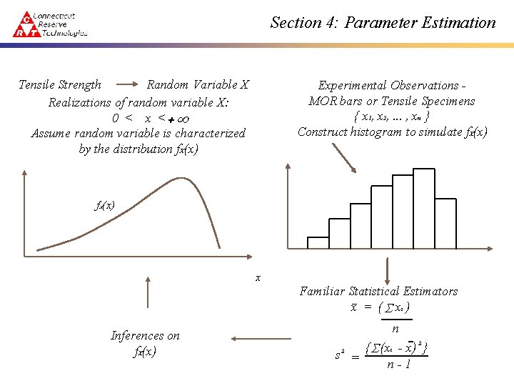
Section 4: Parameter Estimation ESTIMATION THEORY - INTRODUCTION The parameters associated with a distribution must be estimated on the basis of samples obtained from the population the distribution is modeling. The role of sampling as it relates to the statistical inference and parameter estimation is outlined in the figure in the next overhead. The point is to construct a mathematical model that captures the population under study. This requires • inferring the type of distribution that best characterizes the population; and • estimating parameters once the distribution has been established. Thus sampling a population will yield information in order to establish values of the parameters associated with the chosen distribution.

Section 4: Parameter Estimation Tensile Strength Random Variable X Realizations of random variable X: 0 < x < +¥ Assume random variable is characterized by the distribution f. X(x) Experimental Observations MOR bars or Tensile Specimens { x 1, x 2, . . . , xn } Construct histogram to simulate f. X(x) f (x) X x Familiar Statistical Estimators x = ( S xi ) Inferences on f. X(x) n { (xi - x) } s = S n-1 2 2

Section 4: Parameter Estimation “Choosing” a distribution can be somewhat of a qualitative and subjective process. We stress that the physics that underlie a problem should indicate an appropriate choice. However, most times the engineer is left with somehow establishing a rational choice, and too often histograms and their shapes are relied on. However there are quantitative tools that can aid the engineer in his/her selection. These tools are known as goodness-of-fit tests, e. g, • Anderson-Darling Goodness-of-Fit Test Usually these types of tests will only indicate when the engineer chooses badly. For ceramics, the industry has focused on the two parameter Weibull distribution. This is a Type III minimum extreme value statistic. Thus physics and mathematics drive this selection. Once the type of distribution has been made, the next step involves parameter estimation. There are two types of parameter estimation • Point Estimates • Interval Estimates

Section 4: Parameter Estimation Point estimation is concerned with the calculation of a single number, from a sample of observations, that “best” represents the parameters associated with a chosen distribution. Interval estimation goes further and establishes a statement on the confidence in the estimated quantity. The result is the determination of an interval indicating the range wherein the true population parameter is located. This range is associated with a level of confidence. For a given number of samples an increasing interval range increases the level of confidence. Alternatively, increasing the sample size will tend to decrease the interval range for a given level of confidence. Best possible combination is a large confidence and small interval size. The endpoints of the interval range define what is known as “confidence bounds. ”

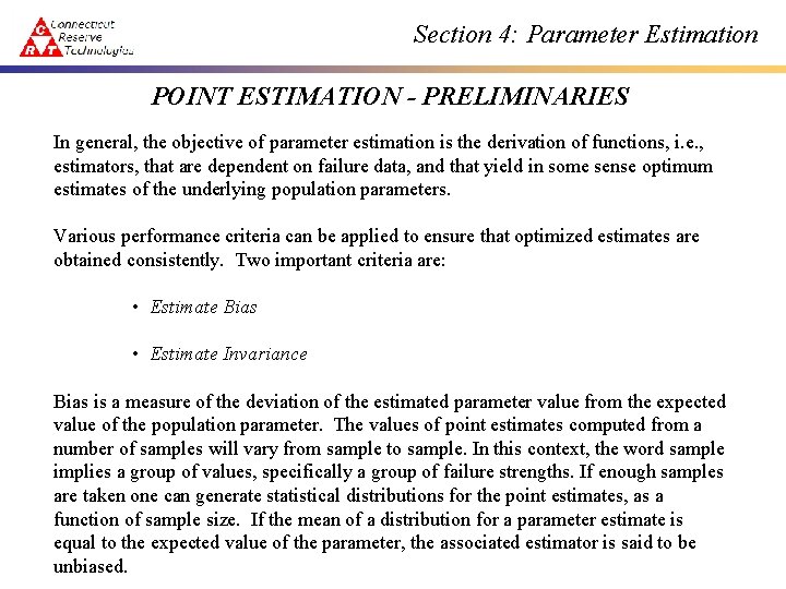
Section 4: Parameter Estimation POINT ESTIMATION - PRELIMINARIES In general, the objective of parameter estimation is the derivation of functions, i. e. , estimators, that are dependent on failure data, and that yield in some sense optimum estimates of the underlying population parameters. Various performance criteria can be applied to ensure that optimized estimates are obtained consistently. Two important criteria are: • Estimate Bias • Estimate Invariance Bias is a measure of the deviation of the estimated parameter value from the expected value of the population parameter. The values of point estimates computed from a number of samples will vary from sample to sample. In this context, the word sample implies a group of values, specifically a group of failure strengths. If enough samples are taken one can generate statistical distributions for the point estimates, as a function of sample size. If the mean of a distribution for a parameter estimate is equal to the expected value of the parameter, the associated estimator is said to be unbiased.

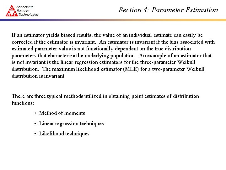
Section 4: Parameter Estimation If an estimator yields biased results, the value of an individual estimate can easily be corrected if the estimator is invariant. An estimator is invariant if the bias associated with estimated parameter value is not functionally dependent on the true distribution parameters that characterize the underlying population. An example of an estimator that is not invariant is the linear regression estimators for the three-parameter Weibull distribution. The maximum likelihood estimator (MLE) for a two-parameter Weibull distribution is invariant. There are three typical methods utilized in obtaining point estimates of distribution functions: • Method of moments • Linear regression techniques • Likelihood techniques

Section 4: Parameter Estimation METHOD OF MOMENTS

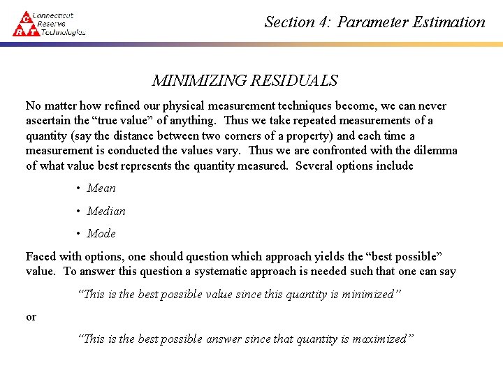
Section 4: Parameter Estimation MINIMIZING RESIDUALS No matter how refined our physical measurement techniques become, we can never ascertain the “true value” of anything. Thus we take repeated measurements of a quantity (say the distance between two corners of a property) and each time a measurement is conducted the values vary. Thus we are confronted with the dilemma of what value best represents the quantity measured. Several options include • Mean • Median • Mode Faced with options, one should question which approach yields the “best possible” value. To answer this question a systematic approach is needed such that one can say “This is the best possible value since this quantity is minimized” or “This is the best possible answer since that quantity is maximized”

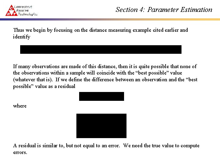
Section 4: Parameter Estimation Thus we begin by focusing on the distance measuring example cited earlier and identify If many observations are made of this distance, then it is quite possible that none of the observations within a sample will coincide with the “best possible” value (whatever that is). If we define the difference between an observation and the “best possible” value as a residual where A residual is similar to, but not equal to an error. We need the true value to compute errors.

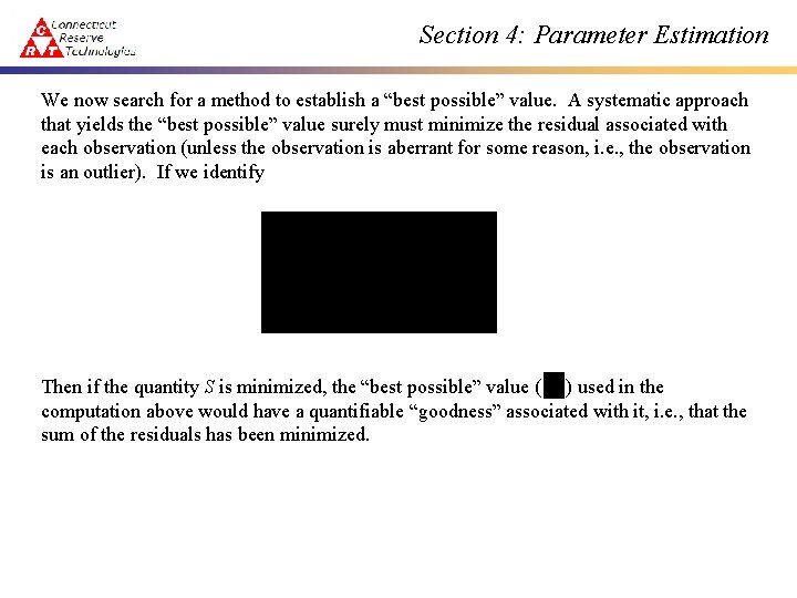
Section 4: Parameter Estimation We now search for a method to establish a “best possible” value. A systematic approach that yields the “best possible” value surely must minimize the residual associated with each observation (unless the observation is aberrant for some reason, i. e. , the observation is an outlier). If we identify Then if the quantity S is minimized, the “best possible” value ( ) used in the computation above would have a quantifiable “goodness” associated with it, i. e. , that the sum of the residuals has been minimized.

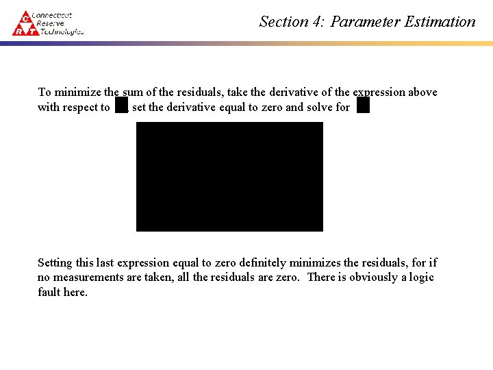
Section 4: Parameter Estimation To minimize the sum of the residuals, take the derivative of the expression above with respect to , set the derivative equal to zero and solve for Setting this last expression equal to zero definitely minimizes the residuals, for if no measurements are taken, all the residuals are zero. There is obviously a logic fault here.

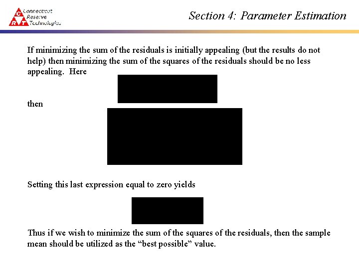
Section 4: Parameter Estimation If minimizing the sum of the residuals is initially appealing (but the results do not help) then minimizing the sum of the squares of the residuals should be no less appealing. Here then Setting this last expression equal to zero yields Thus if we wish to minimize the sum of the squares of the residuals, then the sample mean should be utilized as the “best possible” value.

Section 4: Parameter Estimation Note that we developed this argument in terms of deriving a best possible value for a series of measurements. This concept can be easily extended to estimating values for distribution parameters, where instead of making a “measurement, ” we take a sample from the underlying population. Minimizing the sum of the squares of the residuals is not the only systematic approach in producing the “best possible” estimates of distribution parameters. The maximum likelihood technique is another systematic approach where a “likelihood” is maximized. This technique is described in a later section. In some instances the estimators from various methods coincide, most times they do not. In situations where different approaches produce different estimators (and estimates), then one must choose between the different techniques. The amount of bias produced by an estimator is one measure of assessing efficacy. Additional statistical tools are available.

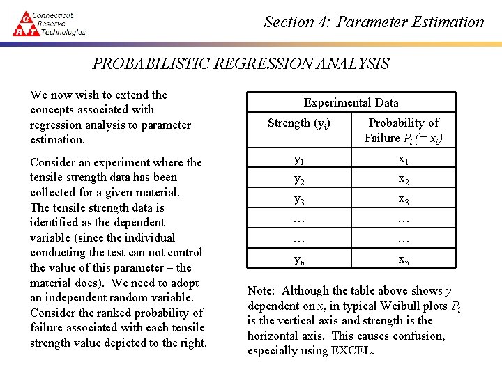
Section 4: Parameter Estimation PROBABILISTIC REGRESSION ANALYSIS We now wish to extend the concepts associated with regression analysis to parameter estimation. Consider an experiment where the tensile strength data has been collected for a given material. The tensile strength data is identified as the dependent variable (since the individual conducting the test can not control the value of this parameter – the material does). We need to adopt an independent random variable. Consider the ranked probability of failure associated with each tensile strength value depicted to the right. Experimental Data Strength (yi) Probability of Failure Pi (= xi) y 1 x 1 y 2 x 2 y 3 x 3 … … yn xn Note: Although the table above shows y dependent on x, in typical Weibull plots Pi is the vertical axis and strength is the horizontal axis. This causes confusion, especially using EXCEL.

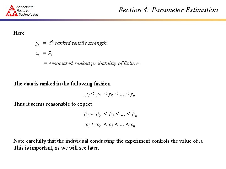
Section 4: Parameter Estimation Here yi = ith ranked tensile strength xi = P i = Associated ranked probability of failure The data is ranked in the following fashion y 1 < y 2 < y 3 <. . . < yn Thus it seems reasonable to expect P 1 < P 2 < P 3 <. . . < Pn x 1 < x 2 < x 3 <. . . < xn Note carefully that the individual conducting the experiment controls the value of n. This is important, as we will see later.

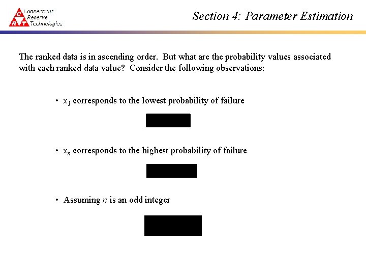
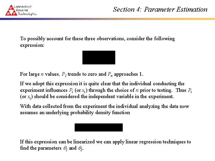
Section 4: Parameter Estimation The ranked data is in ascending order. But what are the probability values associated with each ranked data value? Consider the following observations: • x 1 corresponds to the lowest probability of failure • xn corresponds to the highest probability of failure • Assuming n is an odd integer

Section 4: Parameter Estimation To possibly account for these three observations, consider the following expression: For large n values, P 1 trends to zero and Pn approaches 1. If we adopt this expression it is quite clear that the individual conducting the experiment influences Pi (or xi) through the choice of n prior to testing. Thus Pi (or xi) should be considered the independent variable in the experiment. With data collected from the experiment the individual analyzing the data now assumes an underlying probability density function If this expression can be linearized we can apply linear regression techniques to find the parameters q 1 and q 2.

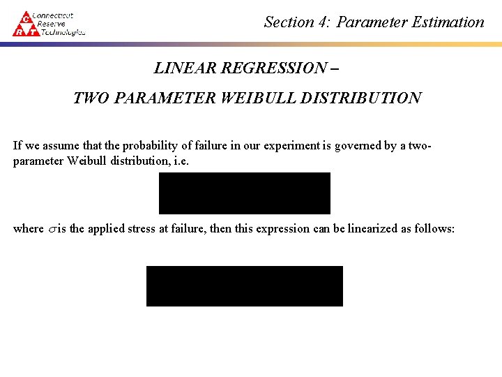
Section 4: Parameter Estimation LINEAR REGRESSION – TWO PARAMETER WEIBULL DISTRIBUTION If we assume that the probability of failure in our experiment is governed by a twoparameter Weibull distribution, i. e. where is the applied stress at failure, then this expression can be linearized as follows:

Section 4: Parameter Estimation If we take Then

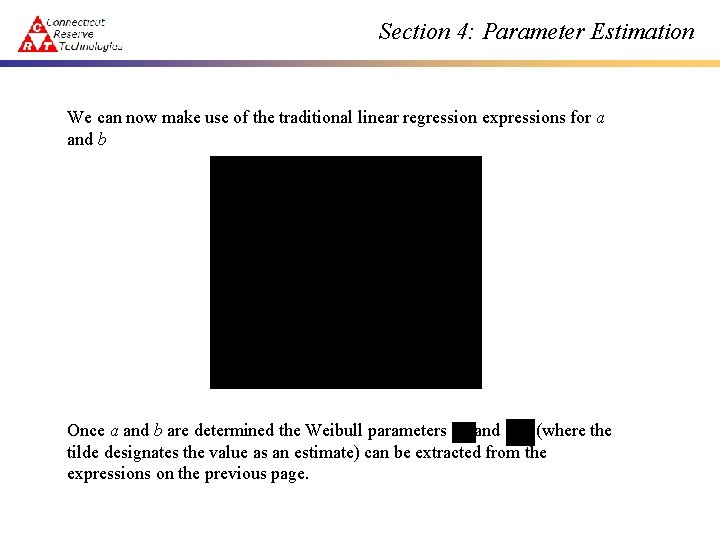
Section 4: Parameter Estimation We can now make use of the traditional linear regression expressions for a and b Once a and b are determined the Weibull parameters and (where the tilde designates the value as an estimate) can be extracted from the expressions on the previous page.

Section 4: Parameter Estimation PROBABILITY OF FAILURE – RANKING SCHEMES A number of ranking schemes for Pi have been proposed in the literature. A mean ranking scheme was introduced in the previous section. In this section a median ranking scheme is discussed. As Johnson (1951) points out, the usual method of statistical inference involves constructing a histogram, from which a smoothed probability density function is derived. However, small sample sizes present difficulties since histograms vary greatly with changes in class intervals. As an alternative to this, ordered statistics were developed whereby ranked failure data is utilized. Consider a sample with five observations, where the observations are arranged in an increasing numerical order. It would seem reasonable to assume that the first observation (lowest value) would represent a value where 20% of the entire population would fall below this value. Thus an estimate for Pi of 20% is assigned this ranked value. Similarly a value of 40%, 60%, 80% and 100% would be assigned to the other ranked observations.

Section 4: Parameter Estimation If we concentrate on the first observation, assuming that 20% of the entire population falls below this value is a fairly far-reaching assumption. This statement can be made for the other four estimate Pi values Thus we will appeal to a statistical estimate of the population fraction that lies below this 20% value. To illustrate the concept, consider a sample of five observations taken from a population whose probability density function and attending distribution parameters are known. This sample of five is repeated four times, and for each sample the data is arranged in ascending order. If the cumulative distribution function for the first value is computed, then F(x 1) = percentage of the population below the value of x 1

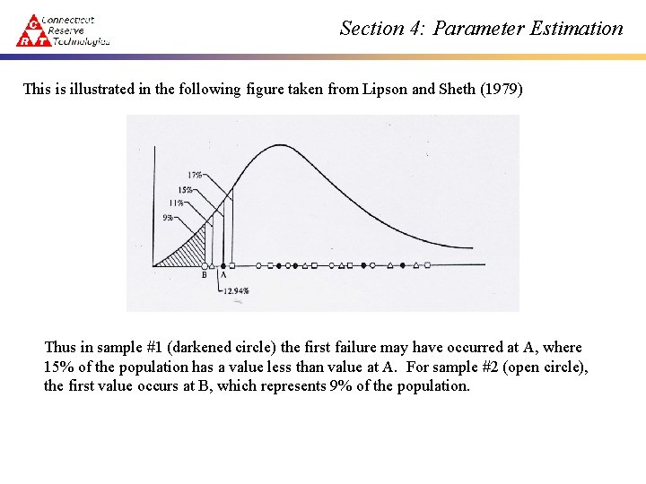
Section 4: Parameter Estimation This is illustrated in the following figure taken from Lipson and Sheth (1979) Thus in sample #1 (darkened circle) the first failure may have occurred at A, where 15% of the population has a value less than value at A. For sample #2 (open circle), the first value occurs at B, which represents 9% of the population.

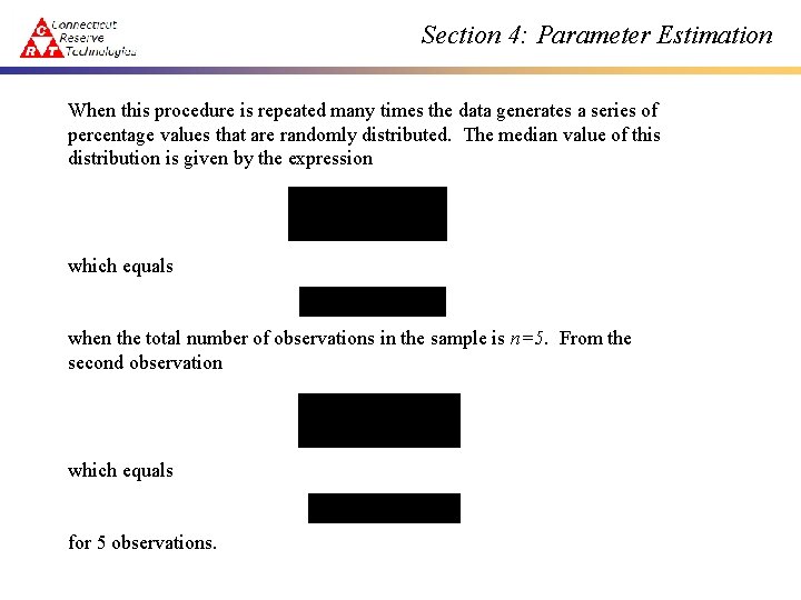
Section 4: Parameter Estimation When this procedure is repeated many times the data generates a series of percentage values that are randomly distributed. The median value of this distribution is given by the expression which equals when the total number of observations in the sample is n=5. From the second observation which equals for 5 observations.

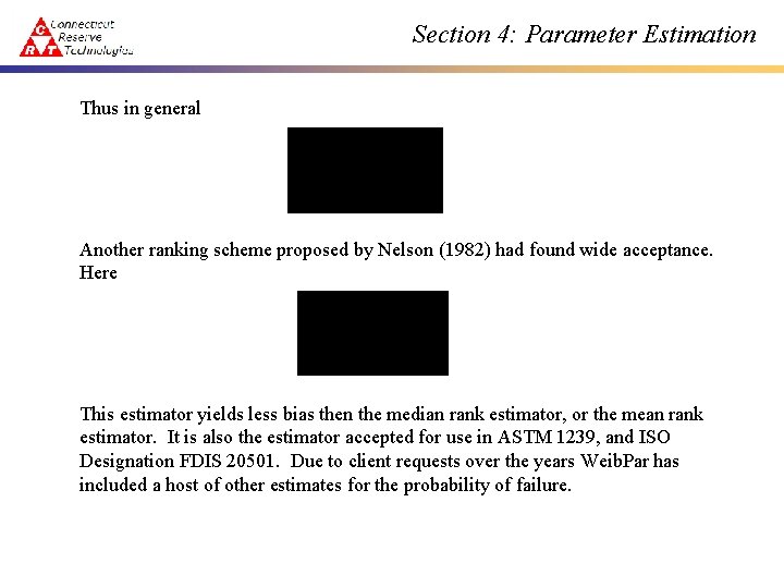
Section 4: Parameter Estimation Thus in general Another ranking scheme proposed by Nelson (1982) had found wide acceptance. Here This estimator yields less bias then the median rank estimator, or the mean rank estimator. It is also the estimator accepted for use in ASTM 1239, and ISO Designation FDIS 20501. Due to client requests over the years Weib. Par has included a host of other estimates for the probability of failure.

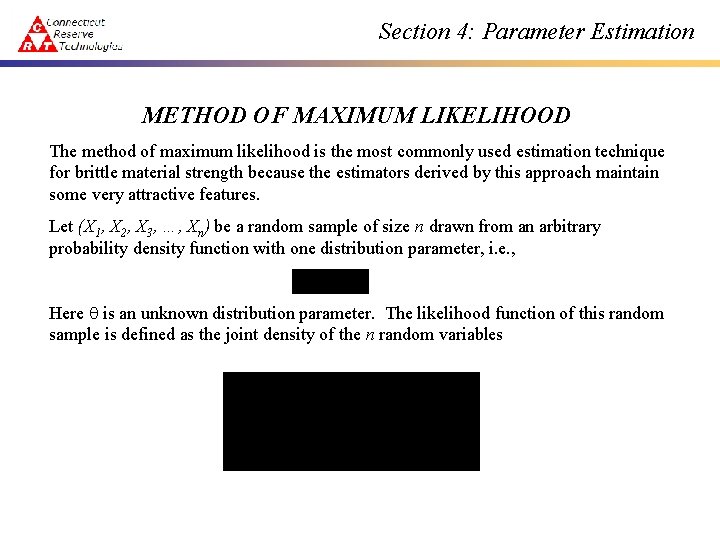
Section 4: Parameter Estimation METHOD OF MAXIMUM LIKELIHOOD The method of maximum likelihood is the most commonly used estimation technique for brittle material strength because the estimators derived by this approach maintain some very attractive features. Let (X 1, X 2, X 3, …, Xn) be a random sample of size n drawn from an arbitrary probability density function with one distribution parameter, i. e. , Here q is an unknown distribution parameter. The likelihood function of this random sample is defined as the joint density of the n random variables

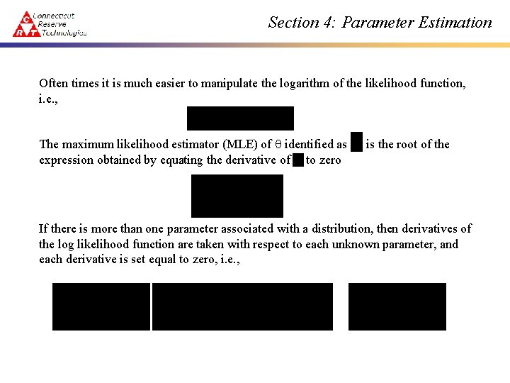
Section 4: Parameter Estimation Often times it is much easier to manipulate the logarithm of the likelihood function, i. e. , The maximum likelihood estimator (MLE) of q identified as expression obtained by equating the derivative of to zero , is the root of the If there is more than one parameter associated with a distribution, then derivatives of the log likelihood function are taken with respect to each unknown parameter, and each derivative is set equal to zero, i. e. ,

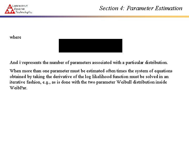
Section 4: Parameter Estimation where And k represents the number of parameters associated with a particular distribution. When more than one parameter must be estimated often times the system of equations obtained by taking the derivative of the log likelihood function must be solved in an iterative fashion, e. g. , as is done with the two parameter Weibull distribution inside Weib. Par.

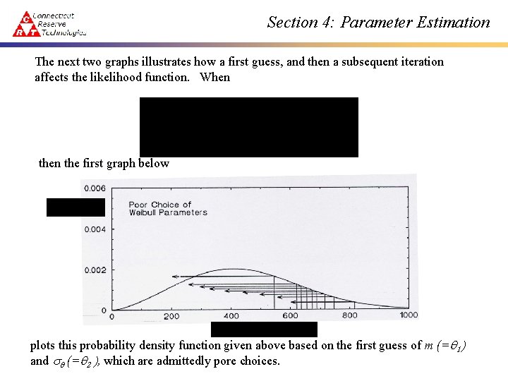
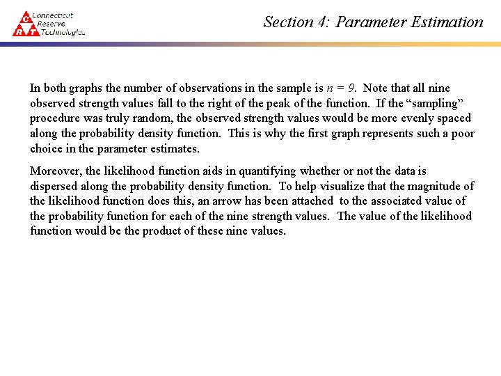
Section 4: Parameter Estimation The next two graphs illustrates how a first guess, and then a subsequent iteration affects the likelihood function. When the first graph below plots this probability density function given above based on the first guess of m (=q 1) and q (=q 2 ), which are admittedly pore choices.

Section 4: Parameter Estimation In both graphs the number of observations in the sample is n = 9. Note that all nine observed strength values fall to the right of the peak of the function. If the “sampling” procedure was truly random, the observed strength values would be more evenly spaced along the probability density function. This is why the first graph represents such a poor choice in the parameter estimates. Moreover, the likelihood function aids in quantifying whether or not the data is dispersed along the probability density function. To help visualize that the magnitude of the likelihood function does this, an arrow has been attached to the associated value of the probability function for each of the nine strength values. The value of the likelihood function would be the product of these nine values.

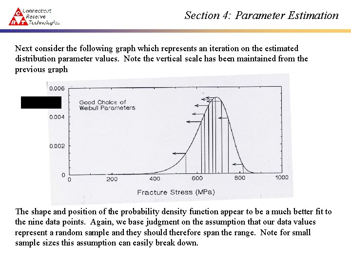
Section 4: Parameter Estimation Next consider the following graph which represents an iteration on the estimated distribution parameter values. Note the vertical scale has been maintained from the previous graph The shape and position of the probability density function appear to be a much better fit to the nine data points. Again, we base judgment on the assumption that our data values represent a random sample and they should therefore span the range. Note for small sample sizes this assumption can easily break down.

Section 4: Parameter Estimation Again, nine arrows point to the associated values of the joint probability density function for each of the nine failure strengths. The product of these nine values represents the value of the likelihood function for this choice of distribution parameters. A simple inspection is sufficient to conclude that the likelihood from the latter iteration is greater than the likelihood from the former. If the latter choice of parameters is considered more acceptable, then this would indicate that obtaining a “best” set of distribution parameters involves maximizing the likelihood function. Two important properties of maximum likelihood estimators 1. Maximum likelihood estimators yield unique solutions 2. Estimates asymptotically converge to the true parameters as the sample size increases

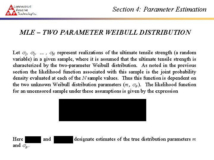
Section 4: Parameter Estimation MLE – TWO PARAMETER WEIBULL DISTRIBUTION Let 1, 2, . . . , N represent realizations of the ultimate tensile strength (a random variable) in a given sample, where it is assumed that the ultimate tensile strength is characterized by the two-parameter Weibull distribution. As noted in the previous section the likelihood function associated with this sample is the joint probability density evaluated at each of the N sample values. Thus this function is dependent on the two unknown Weibull distribution parameters (m, q ). The likelihood function for an uncensored sample under these assumptions is given by the expression Here and q. and designate estimates of the true distribution parameters m

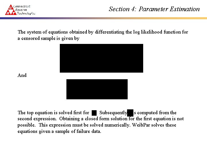
Section 4: Parameter Estimation The system of equations obtained by differentiating the log likelihood function for a censored sample is given by And The top equation is solved first for. Subsequently is computed from the second expression. Obtaining a closed form solution for the first equation is not possible. This expression must be solved numerically. Weib. Par solves these equations given a sample of failure data.

Section 4: Parameter Estimation EXAMPLE - SINGLE FLAW DISTRIBUTION Weib. Par – Uncen. dat

Section 4: Parameter Estimation PARAMETER ESTIMATE BIAS A certain amount of intrinsic variability occurs due to sampling error. This error is associated with the fact that only a limited number of observations are taken from an infinite (assumed) population. Bias - Deviation of the expected value of the estimated parameter from the true parameter. This is the tendency of a particular estimator to give consistently high or consistently low estimates relative to the true value. Once it is recognized that the estimates of the Weibull modulus and characteristic strength will vary from sample to sample, these estimates can be treated as random variables (i. e. , statistics).

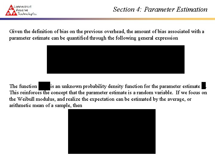
Section 4: Parameter Estimation Given the definition of bias on the previous overhead, the amount of bias associated with a parameter estimate can be quantified through the following general expression The function is an unknown probability density function for the parameter estimate. This reinforces the concept that the parameter estimate is a random variable. If we focus on the Weibull modulus, and realize the expectation can be estimated by the average, or arithmetic mean of a sample, then

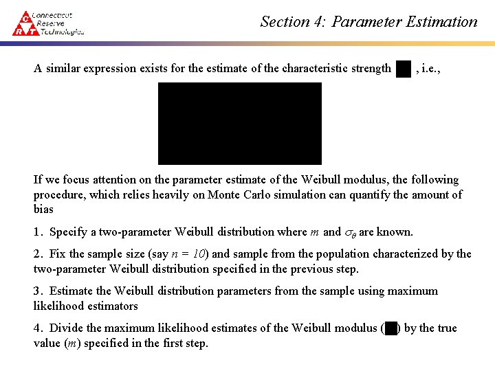
Section 4: Parameter Estimation A similar expression exists for the estimate of the characteristic strength , i. e. , If we focus attention on the parameter estimate of the Weibull modulus, the following procedure, which relies heavily on Monte Carlo simulation can quantify the amount of bias 1. Specify a two-parameter Weibull distribution where m and q are known. 2. Fix the sample size (say n = 10) and sample from the population characterized by the two-parameter Weibull distribution specified in the previous step. 3. Estimate the Weibull distribution parameters from the sample using maximum likelihood estimators 4. Divide the maximum likelihood estimates of the Weibull modulus ( ) by the true value (m) specified in the first step.

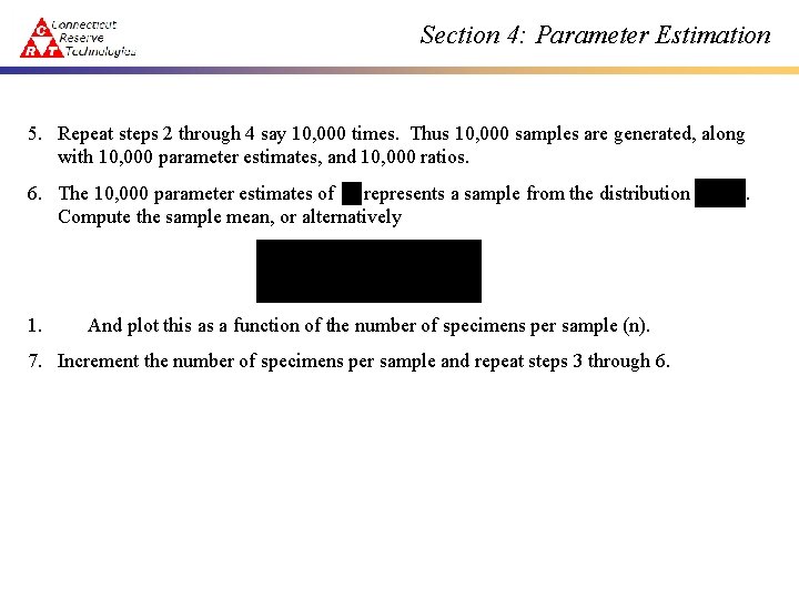
Section 4: Parameter Estimation 5. Repeat steps 2 through 4 say 10, 000 times. Thus 10, 000 samples are generated, along with 10, 000 parameter estimates, and 10, 000 ratios. 6. The 10, 000 parameter estimates of represents a sample from the distribution Compute the sample mean, or alternatively 1. And plot this as a function of the number of specimens per sample (n). 7. Increment the number of specimens per sample and repeat steps 3 through 6. .

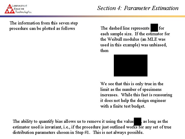
Section 4: Parameter Estimation The information from this seven step procedure can be plotted as follows The dashed line represents for each sample size. If the estimator for the Weibull modulus (an MLE was used in this example) was unbiased, then We see that this is only true in the limit as the number of specimens increases. While this fact is reassuring it does not help the design engineer with a finite test budget. The ability to quantify bias allows us to remove it using the value , as long as the estimator used is invariant, i. e. , if the procedure just outlined works for any set of true distribution parameters chosen in Step #1. This is not always possible.

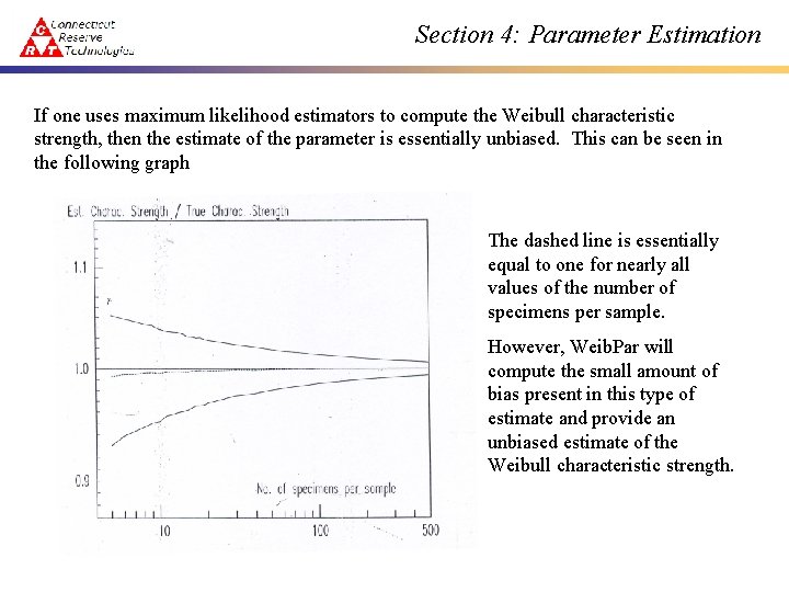
Section 4: Parameter Estimation If one uses maximum likelihood estimators to compute the Weibull characteristic strength, then the estimate of the parameter is essentially unbiased. This can be seen in the following graph The dashed line is essentially equal to one for nearly all values of the number of specimens per sample. However, Weib. Par will compute the small amount of bias present in this type of estimate and provide an unbiased estimate of the Weibull characteristic strength.

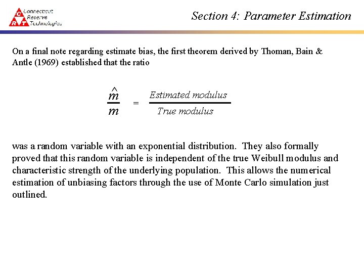
Section 4: Parameter Estimation On a final note regarding estimate bias, the first theorem derived by Thoman, Bain & Antle (1969) established that the ratio ^ m m = Estimated modulus True modulus was a random variable with an exponential distribution. They also formally proved that this random variable is independent of the true Weibull modulus and characteristic strength of the underlying population. This allows the numerical estimation of unbiasing factors through the use of Monte Carlo simulation just outlined.

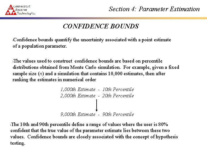
Section 4: Parameter Estimation CONFIDENCE BOUNDS Confidence bounds quantify the uncertainty associated with a point estimate of a population parameter. l The values used to construct confidence bounds are based on percentile distributions obtained from Monte Carlo simulation. For example, given a fixed sample size (n) and a simulation that contains 10, 000 estimates, then after ranking the estimates in numerical order l 1, 000 th Estimate - 10 th Percentile 2, 000 th Estimate - 20 th Percentile 9, 000 th Estimate - 90 th Percentile The 10 th and 90 th percentile define a range of values where the user is 80% confident that the true value of the parameter estimate lies between these two values. Confidence bounds are closely associated with the concept of hypothesis testing. l

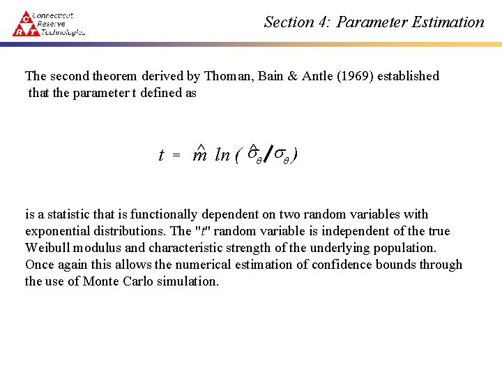
Section 4: Parameter Estimation The second theorem derived by Thoman, Bain & Antle (1969) established that the parameter t defined as t = ^ ln ( ^q q ) m is a statistic that is functionally dependent on two random variables with exponential distributions. The "t" random variable is independent of the true Weibull modulus and characteristic strength of the underlying population. Once again this allows the numerical estimation of confidence bounds through the use of Monte Carlo simulation.

Section 4: Parameter Estimation EXAMPLE - SINGLE FLAW DISTRIBUTION Weib. Par – Uncen. dat (focus on unbiased values and confidence bounds)

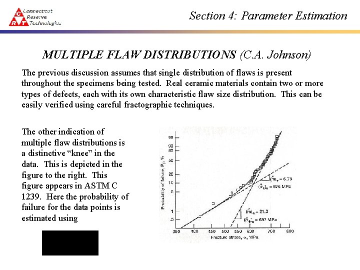
Section 4: Parameter Estimation MULTIPLE FLAW DISTRIBUTIONS (C. A. Johnson) The previous discussion assumes that single distribution of flaws is present throughout the specimens being tested. Real ceramic materials contain two or more types of defects, each with its own characteristic flaw size distribution. This can be easily verified using careful fractographic techniques. The other indication of multiple flaw distributions is a distinctive “knee” in the data. This is depicted in the figure to the right. This figure appears in ASTM C 1239. Here the probability of failure for the data points is estimated using

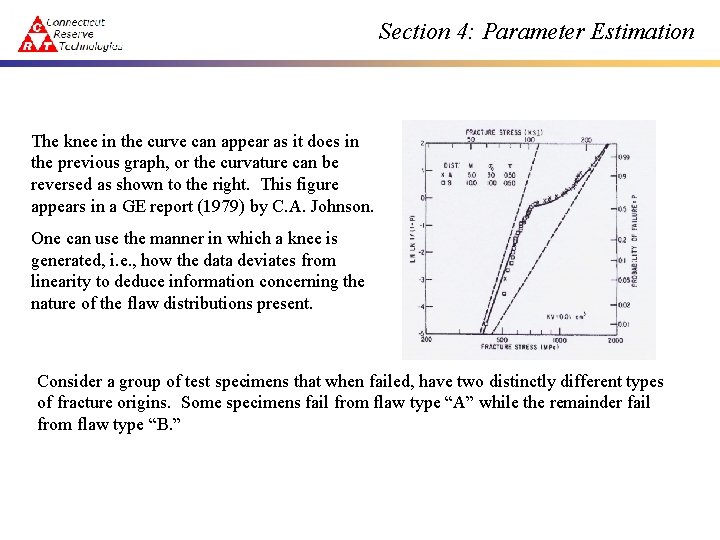
Section 4: Parameter Estimation The knee in the curve can appear as it does in the previous graph, or the curvature can be reversed as shown to the right. This figure appears in a GE report (1979) by C. A. Johnson. One can use the manner in which a knee is generated, i. e. , how the data deviates from linearity to deduce information concerning the nature of the flaw distributions present. Consider a group of test specimens that when failed, have two distinctly different types of fracture origins. Some specimens fail from flaw type “A” while the remainder fail from flaw type “B. ”

Section 4: Parameter Estimation There at least three ways in which these two flaw populations are present in the test specimens, i. e. , the sample. • Both flaw distributions are present in every test specimen. This is known as “Concurrent Flaw Populations. ” • Within a group of specimens any given specimen may contain flaws from distribution A, or from distribution B, but not from both. This is known as “Mutually Exclusive Flaw Populations. ” • Within a group of specimens, flaw distribution A may be present in all specimens, while distribution B may be present in only some test specimens. This is known as “Partially Concurrent Flaw Populations. ” A larger number of cases must be considered than three above if more than two flaw distributions are active.

Section 4: Parameter Estimation Examples of the three types of flaw distributions are as follows. Concurrent Flaw Distributions – A group of test specimens machined from a ceramic billet which contains defects distributed throughout the volume. Each specimen then contains both machining flaws on the surface and volume defects interior to the test specimen. Exclusive Flaw Distributions – A group of test specimens comprised of two subgroups purchased from two different manufacturer. Partially Concurrent Distributions - A group of pressed and sintered test specimens which were all sintered in the same furnace, but could not be sintered in a single furnace cycle. The specimens sintered at the longer cycle would contain elongated grains (considered a deleterious flaws) and all the specimens would have strength degrading inclusions present from the powder preparation. The parameter estimation methods presented here assumes that if multiple flaw populations are present, then they are concurrent flaw distributions. As indicated above, partially concurrent distributions point to processing methods that have not , or are not mature. In addition, it is quite typical for a manufacturer of ceramic components to identify one material supplier, and this would minimize the presence of exclusive flaw distributions.

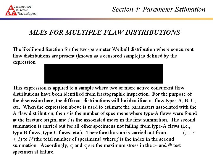
Section 4: Parameter Estimation MLEs FOR MULTIPLE FLAW DISTRIBUTIONS The likelihood function for the two-parameter Weibull distribution where concurrent flaw distributions are present (known as a censored sample) is defined by the expression This expression is applied to a sample where two or more active concurrent flaw distributions have been identified from fractographic inspection. For the purpose of the discussion here, the different distributions will be identified as flaw types A, B, C, etc. When the expression above is used to estimate the parameters associated with the A flaw distribution, then r is the number of specimens where type-A flaws were found at the fracture origin, and i is the associated index in the first summation. The second summation is carried out for all other specimens not failing from type-A flaws (i. e. , type-B flaws, type-C flaws, etc. ). Therefore the sum is carried out from (j = r + 1) to N (the total number of specimens) where j is the index in the second summation. Accordingly, σi and σj are the maximum stress in the ith and jth test specimen at failure.

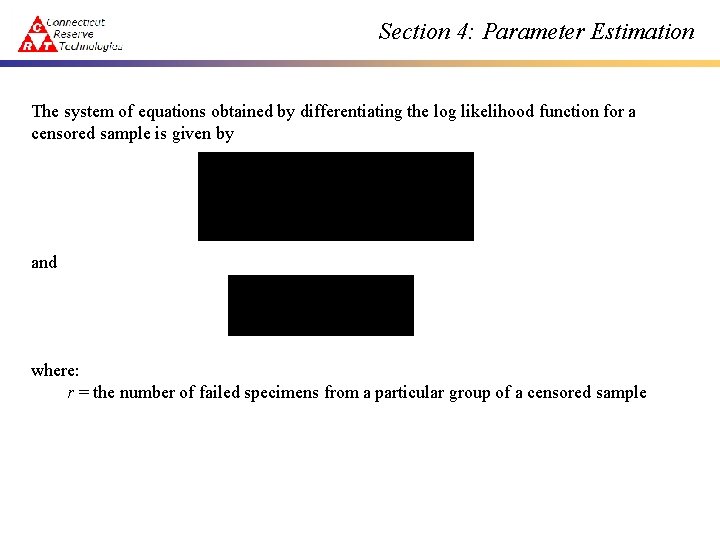
Section 4: Parameter Estimation The system of equations obtained by differentiating the log likelihood function for a censored sample is given by and where: r = the number of failed specimens from a particular group of a censored sample

Section 4: Parameter Estimation EXAMPLE - MULTIPLE FLAW DISTRIBUTIONS

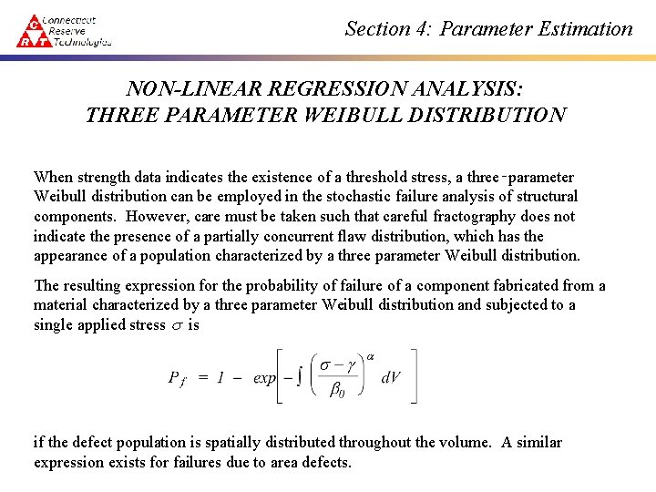
Section 4: Parameter Estimation NON-LINEAR REGRESSION ANALYSIS: THREE PARAMETER WEIBULL DISTRIBUTION When strength data indicates the existence of a threshold stress, a three‑parameter Weibull distribution can be employed in the stochastic failure analysis of structural components. However, care must be taken such that careful fractography does not indicate the presence of a partially concurrent flaw distribution, which has the appearance of a population characterized by a three parameter Weibull distribution. The resulting expression for the probability of failure of a component fabricated from a material characterized by a three parameter Weibull distribution and subjected to a single applied stress is if the defect population is spatially distributed throughout the volume. A similar expression exists for failures due to area defects.

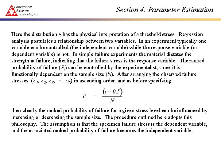
Section 4: Parameter Estimation Here the distribution g has the physical interpretation of a threshold stress. Regression analysis postulates a relationship between two variables. In an experiment typically one variable can be controlled (the independent variable) while the response variable (or dependent variable) is not. In simple failure experiments the material dictates the strength at failure, indicating that the failure stress is the response variable. The ranked probability of failure (Pi) can be controlled by the experimentalist, since it is functionally dependent on the sample size (N). After arranging the observed failure stresses ( 1, 2, 3, , N) in ascending order, and as before specifying then clearly the ranked probability of failure for a given stress level can be influenced by increasing or decreasing the sample size. The procedure outlined here adopts this philosophy. The assumption is that the specimen failure stress is the dependent variable, and the associated ranked probability of failure becomes the independent variable.

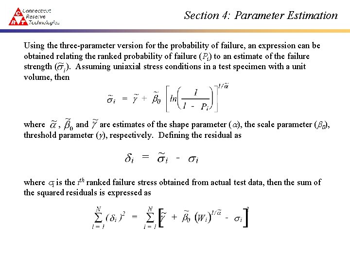
Section 4: Parameter Estimation Using the three-parameter version for the probability of failure, an expression can be obtained relating the ranked probability of failure (Pi) to an estimate of the failure strength ( ). Assuming uniaxial stress conditions in a test specimen with a unit volume, then where , and are estimates of the shape parameter (a), the scale parameter (b 0), threshold parameter (g), respectively. Defining the residual as where i is the ith ranked failure stress obtained from actual test data, then the sum of the squared residuals is expressed as

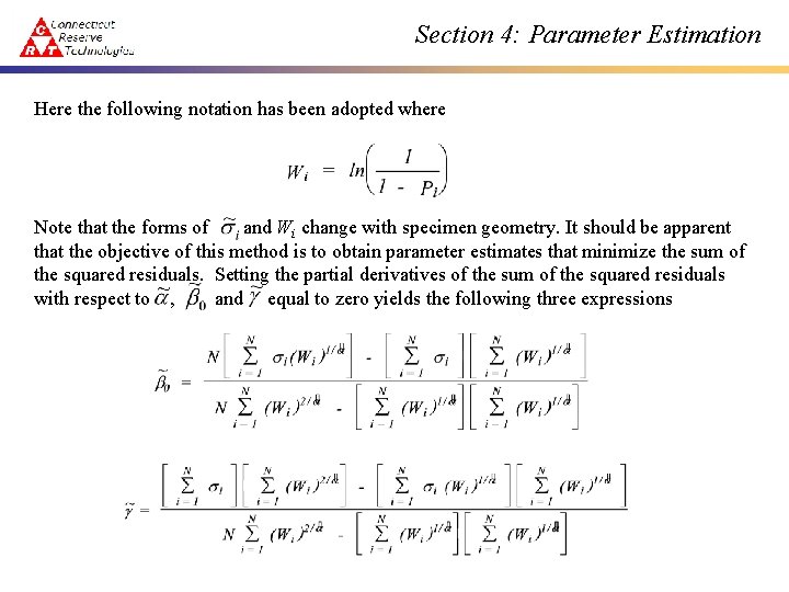
Section 4: Parameter Estimation Here the following notation has been adopted where Note that the forms of and Wi change with specimen geometry. It should be apparent that the objective of this method is to obtain parameter estimates that minimize the sum of the squared residuals. Setting the partial derivatives of the sum of the squared residuals with respect to , and equal to zero yields the following three expressions

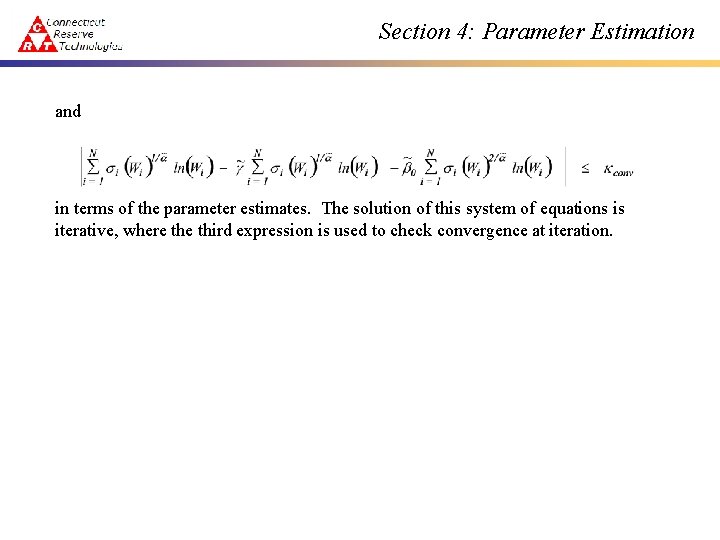
Section 4: Parameter Estimation and in terms of the parameter estimates. The solution of this system of equations is iterative, where third expression is used to check convergence at iteration.

Section 4: Parameter Estimation EXAMPLE – THREE PARAMETER WEIBULL DISTRIBUTION

Section 4: Parameter Estimation

Section 4: Parameter Estimation