Managerial Economics Production Theory and Estimation The Organization

Managerial Economics Production Theory and Estimation

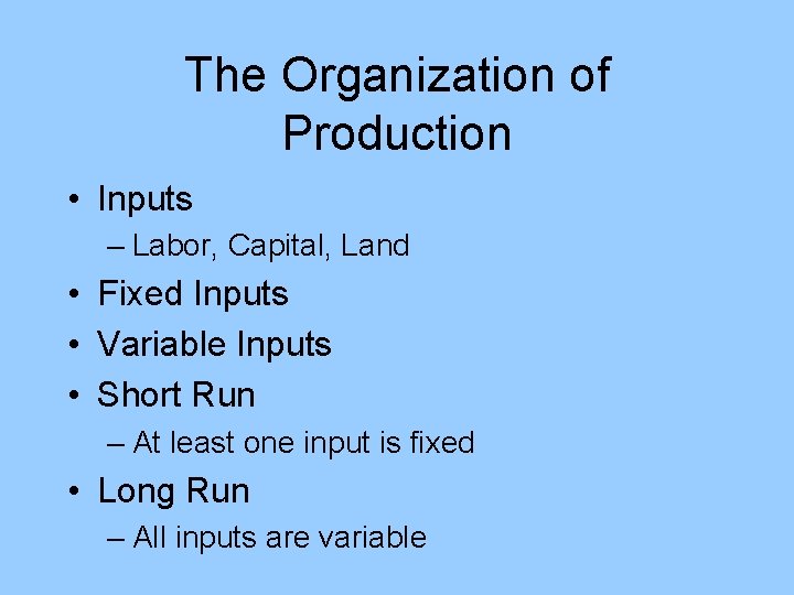
The Organization of Production • Inputs – Labor, Capital, Land • Fixed Inputs • Variable Inputs • Short Run – At least one input is fixed • Long Run – All inputs are variable

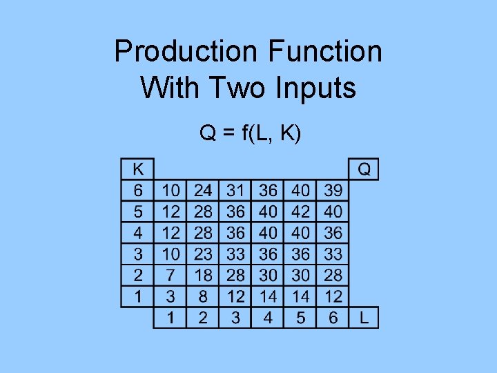
Production Function With Two Inputs Q = f(L, K)

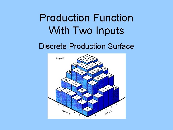
Production Function With Two Inputs Discrete Production Surface

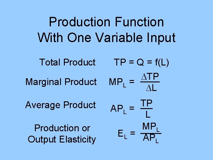
Production Function With One Variable Input Total Product Marginal Product Average Production or Output Elasticity TP = Q = f(L) TP MPL = L TP APL = L MPL EL = AP L

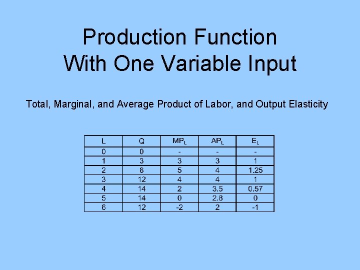
Production Function With One Variable Input Total, Marginal, and Average Product of Labor, and Output Elasticity

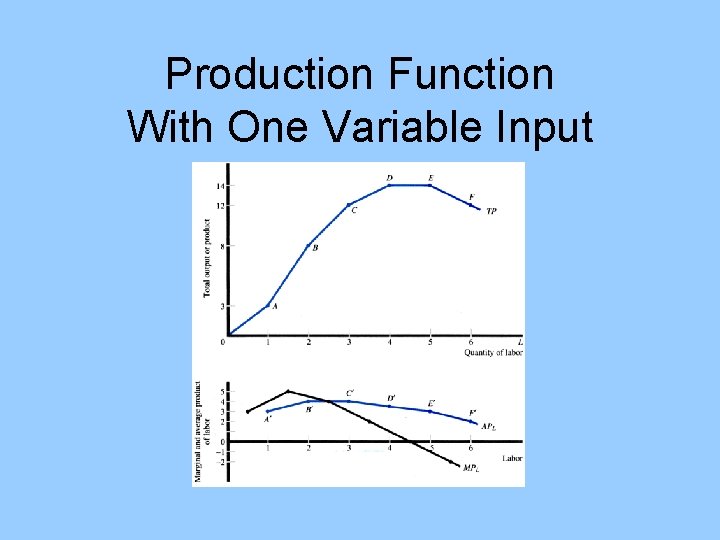
Production Function With One Variable Input

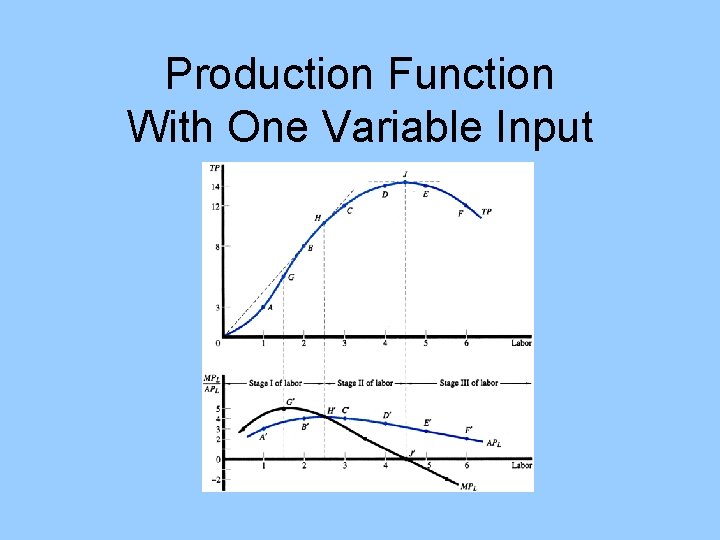
Production Function With One Variable Input

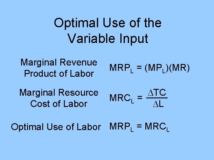
Optimal Use of the Variable Input Marginal Revenue Product of Labor MRPL = (MPL)(MR) Marginal Resource Cost of Labor TC MRCL = L Optimal Use of Labor MRPL = MRCL

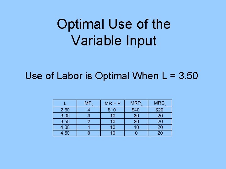
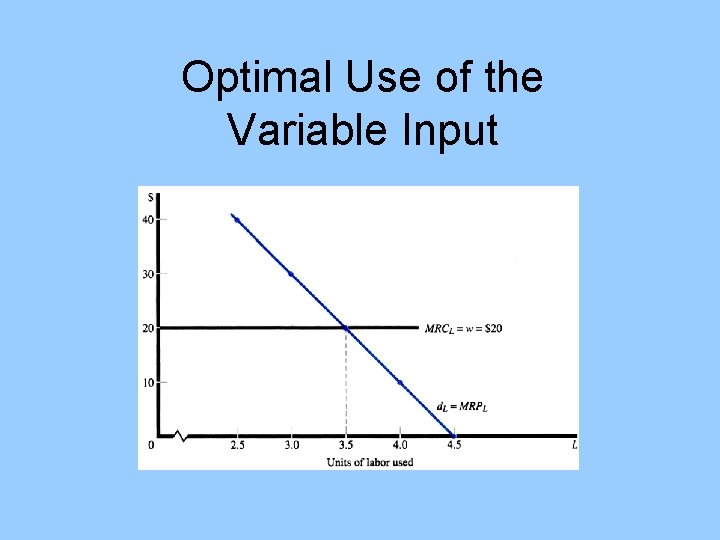
Optimal Use of the Variable Input Use of Labor is Optimal When L = 3. 50

Optimal Use of the Variable Input

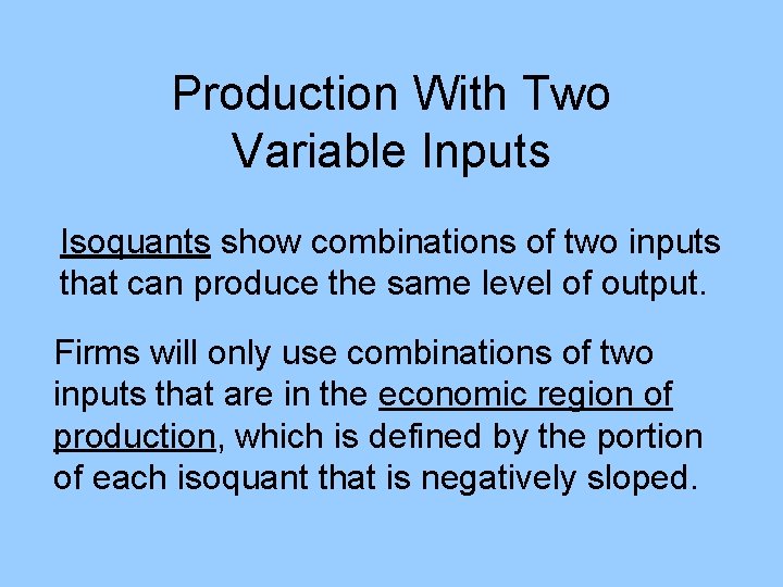
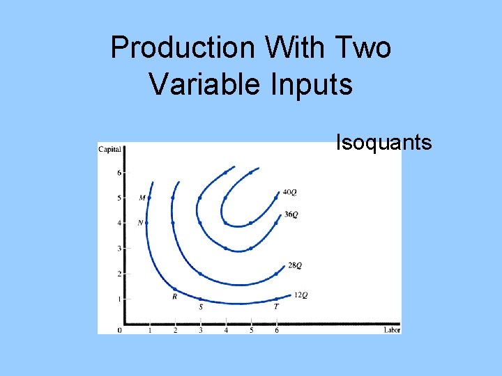
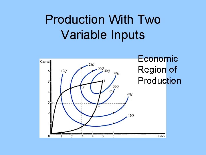
Production With Two Variable Inputs Isoquants show combinations of two inputs that can produce the same level of output. Firms will only use combinations of two inputs that are in the economic region of production, which is defined by the portion of each isoquant that is negatively sloped.

Production With Two Variable Inputs Isoquants

Production With Two Variable Inputs Economic Region of Production

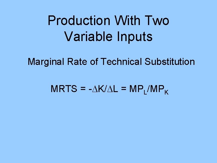
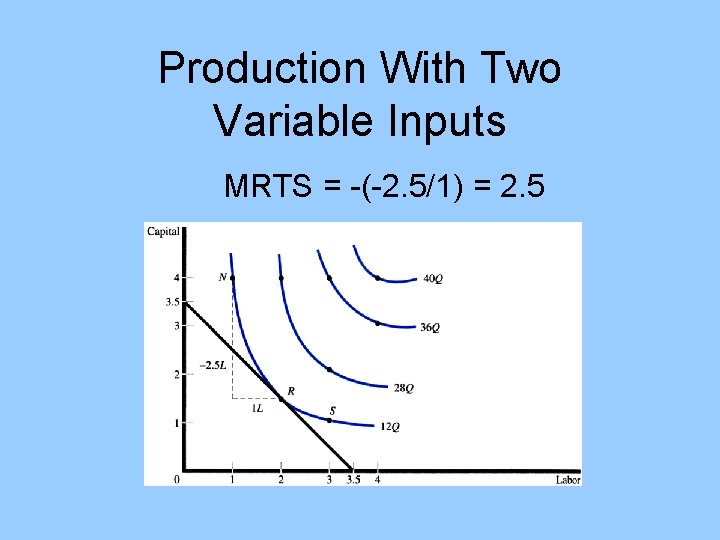
Production With Two Variable Inputs Marginal Rate of Technical Substitution MRTS = - K/ L = MPL/MPK

Production With Two Variable Inputs MRTS = -(-2. 5/1) = 2. 5

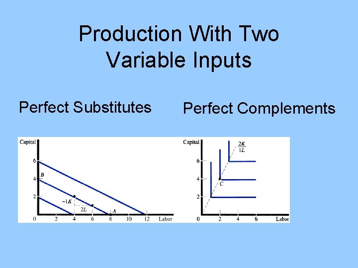
Production With Two Variable Inputs Perfect Substitutes Perfect Complements

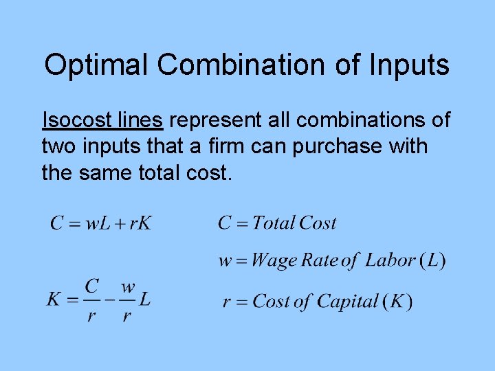
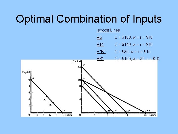
Optimal Combination of Inputs Isocost lines represent all combinations of two inputs that a firm can purchase with the same total cost.

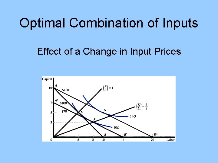
Optimal Combination of Inputs Isocost Lines AB C = $100, w = r = $10 A’B’ C = $140, w = r = $10 A’’B’’ C = $80, w = r = $10 AB* C = $100, w = $5, r = $10

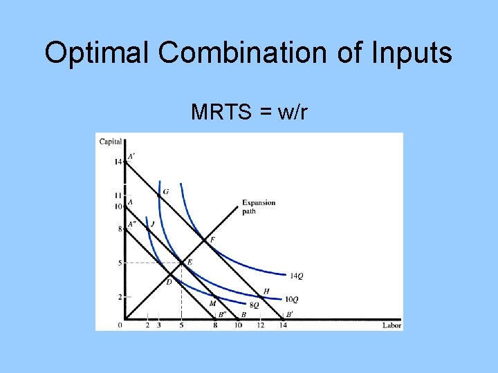
Optimal Combination of Inputs MRTS = w/r

Optimal Combination of Inputs Effect of a Change in Input Prices

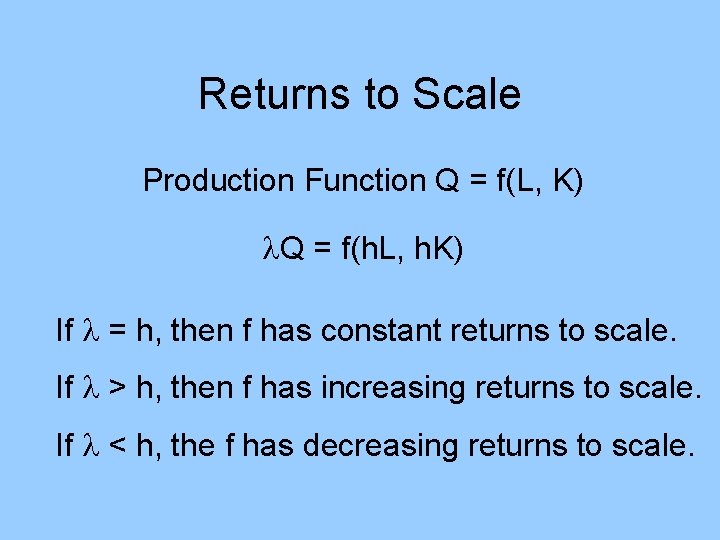
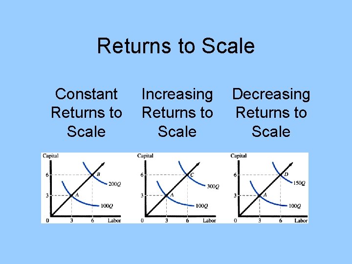
Returns to Scale Production Function Q = f(L, K) Q = f(h. L, h. K) If = h, then f has constant returns to scale. If > h, then f has increasing returns to scale. If < h, the f has decreasing returns to scale.

Returns to Scale Constant Returns to Scale Increasing Returns to Scale Decreasing Returns to Scale

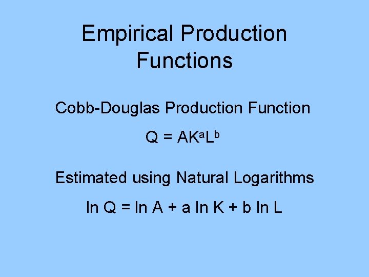
Empirical Production Functions Cobb-Douglas Production Function Q = AKa. Lb Estimated using Natural Logarithms ln Q = ln A + a ln K + b ln L