CLASSIFICATION OF PARAMETER ESTIMATION AND INVERSE PROBLEMS Scaling

CLASSIFICATION OF PARAMETER ESTIMATION AND INVERSE PROBLEMS Scaling and superposition properties that characterize linear systems are given. linear and nonlinear mathematical models. Examples of discrete and continuous linear and nonlinear parameter estimation problems. solution existence, uniqueness, and instability.

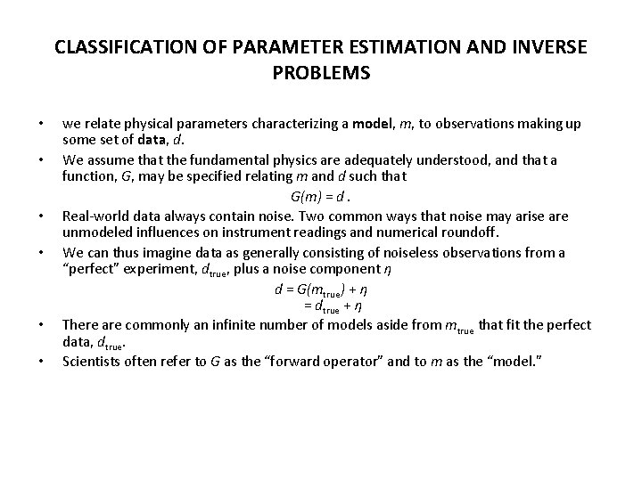
CLASSIFICATION OF PARAMETER ESTIMATION AND INVERSE PROBLEMS • • • we relate physical parameters characterizing a model, m, to observations making up some set of data, d. We assume that the fundamental physics are adequately understood, and that a function, G, may be specified relating m and d such that G(m) = d. Real-world data always contain noise. Two common ways that noise may arise are unmodeled influences on instrument readings and numerical roundoff. We can thus imagine data as generally consisting of noiseless observations from a “perfect” experiment, dtrue, plus a noise component η d = G(mtrue) + η = dtrue + η There are commonly an infinite number of models aside from mtrue that fit the perfect data, dtrue. Scientists often refer to G as the “forward operator” and to m as the “model. ”

forward problem and inverse problem • • • The forward problem is to find d given m. Computing G(m) might involve solving a differential equation, evaluating an integral equation, or applying an algorithm to m for which there is no explicit analytical formulation. The inverse problem of finding m given d. We want to determine a finite number of parameters, n, that define a model. The parameters may define a physical entity directly (e. g. , density, voltage, seismic velocity), or may be coefficients or other constants in a functional relationship that describes a physical process.

discrete inverse problems and continuous inverse problem • • • we can express the model parameters as an n element vector m. Similarly, if there a finite number of data points then we can express the data as an m element vector d. Such problems are called discrete inverse problems or parameter estimation problems. A general parameter estimation problem can be written as a system of equations G(m) = d. Alternatively, where the model and data are functions of continuous variables, such as time or space, the task of estimating m from d is called a continuous inverse problem.

parameter estimation problems and inverse problems • • • We will generally refer to problems with small numbers of parameters as “parameter estimation problems. ” Problems with a larger number of parameters, and which will often require the application of additional stabilizing constraints, will be referred to as “inverse problems. ” The need for stabilizing solution constraints arises because the associated systems of equations or operations are ill-conditioned. In both parameter estimation and inverse problems we solve for a set of parameters that characterize a model. In practice, what is most important is the distinction between ill-conditioned and well-conditioned parameter estimation problems.

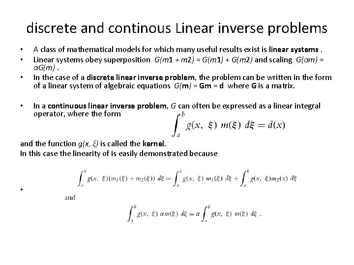
discrete and continous Linear inverse problems • • A class of mathematical models for which many useful results exist is linear systems. Linear systems obey superposition G(m 1 + m 2) = G(m 1) + G(m 2) and scaling G(αm) = αG(m). In the case of a discrete linear inverse problem, the problem can be written in the form of a linear system of algebraic equations G(m) = Gm = d where G is a matrix. In a continuous linear inverse problem, G can often be expressed as a linear integral operator, where the form and the function g(x, ξ) is called the kernel. In this case the linearity of is easily demonstrated because •

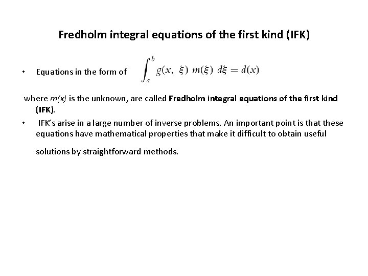
Fredholm integral equations of the first kind (IFK) • Equations in the form of where m(x) is the unknown, are called Fredholm integral equations of the first kind (IFK). • IFK’s arise in a large number of inverse problems. An important point is that these equations have mathematical properties that make it difficult to obtain useful solutions by straightforward methods.

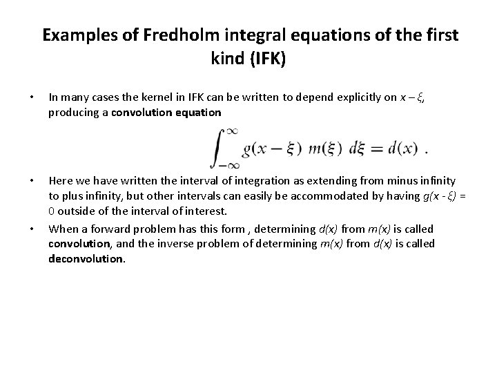
Examples of Fredholm integral equations of the first kind (IFK) • In many cases the kernel in IFK can be written to depend explicitly on x – ξ, producing a convolution equation • Here we have written the interval of integration as extending from minus infinity to plus infinity, but other intervals can easily be accommodated by having g(x - ξ) = 0 outside of the interval of interest. When a forward problem has this form , determining d(x) from m(x) is called convolution, and the inverse problem of determining m(x) from d(x) is called deconvolution. •

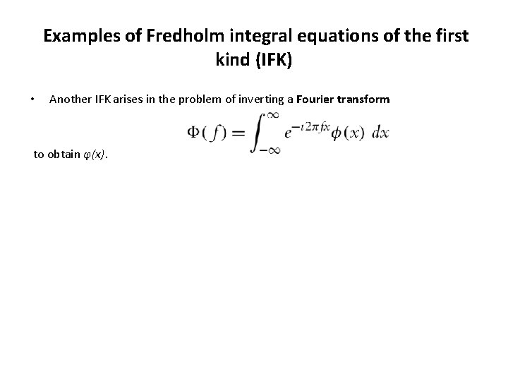
Examples of Fredholm integral equations of the first kind (IFK) • Another IFK arises in the problem of inverting a Fourier transform to obtain φ(x).

Linear and non-linear geophysical inverse problems • • • linearity arises in many interesting physical problems. An important geophysical example of this kind is seismic wave propagation, where the stresses associated with elastic wavefields are often very small relative to the elastic moduli of rocks. This creates only small strains and a very nearly linear stress-strain relationship. Because of this, seismic wavefield problems in many useful circumstances obey superposition and scaling. Other physical fields, such as gravity and magnetism, also have effectively linear physics at the field strengths typically encountered in geophysics. Nonlinear mathematical models arise when model parameters have an inherently nonlinear relationship with respect to data. This situation occurs, for example, in electromagnetic field problems where we wish to relate geometric model parameters such as layer thicknesses to observed field properties.

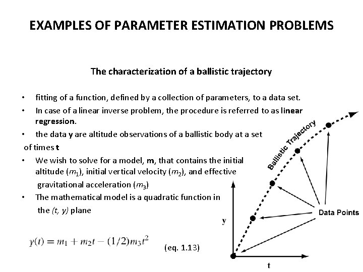
EXAMPLES OF PARAMETER ESTIMATION PROBLEMS The characterization of a ballistic trajectory fitting of a function, defined by a collection of parameters, to a data set. In case of a linear inverse problem, the procedure is referred to as linear regression. • the data y are altitude observations of a ballistic body at a set of times t • We wish to solve for a model, m, that contains the initial altitude (m 1), initial vertical velocity (m 2), and effective gravitational acceleration (m 3) • The mathematical model is a quadratic function in the (t, y) plane • • (eq. 1. 13)

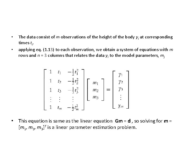
• • The data consist of m observations of the height of the body yi at corresponding times ti. applying eq. (1. 13) to each observation, we obtain a system of equations with m rows and n = 3 columns that relates the data yi to the model parameters, mj • This equation is same as the linear equation Gm = d , so solving for m = [m 1, m 2, m 3]T is a linear parameter estimation problem.

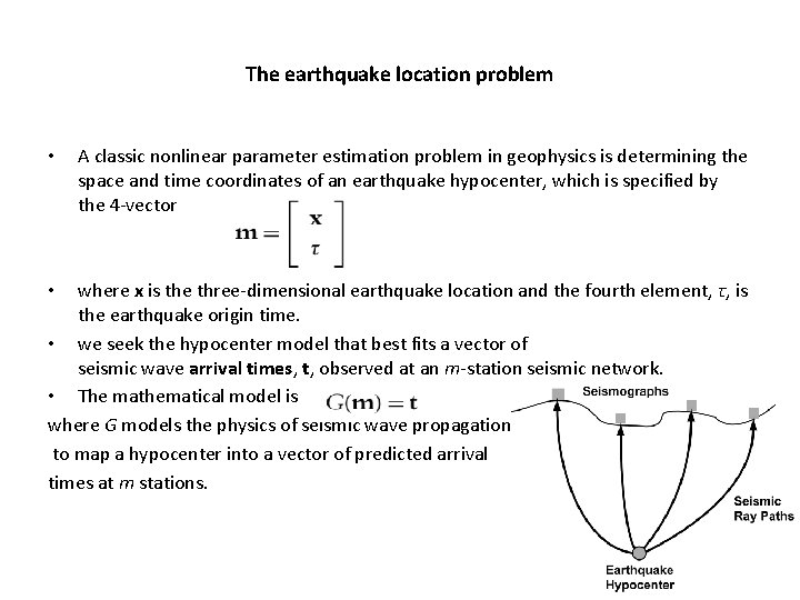
The earthquake location problem • A classic nonlinear parameter estimation problem in geophysics is determining the space and time coordinates of an earthquake hypocenter, which is specified by the 4 -vector where x is the three-dimensional earthquake location and the fourth element, τ, is the earthquake origin time. • we seek the hypocenter model that best fits a vector of seismic wave arrival times, t, observed at an m-station seismic network. • The mathematical model is where G models the physics of seismic wave propagation to map a hypocenter into a vector of predicted arrival times at m stations. •

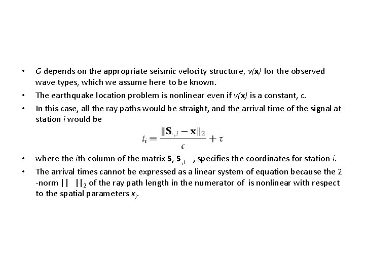
• • • G depends on the appropriate seismic velocity structure, v(x) for the observed wave types, which we assume here to be known. The earthquake location problem is nonlinear even if v(x) is a constant, c. In this case, all the ray paths would be straight, and the arrival time of the signal at station i would be where the ith column of the matrix S, S·, I , specifies the coordinates for station i. The arrival times cannot be expressed as a linear system of equation because the 2 -norm || ||2 of the ray path length in the numerator of is nonlinear with respect to the spatial parameters xi.

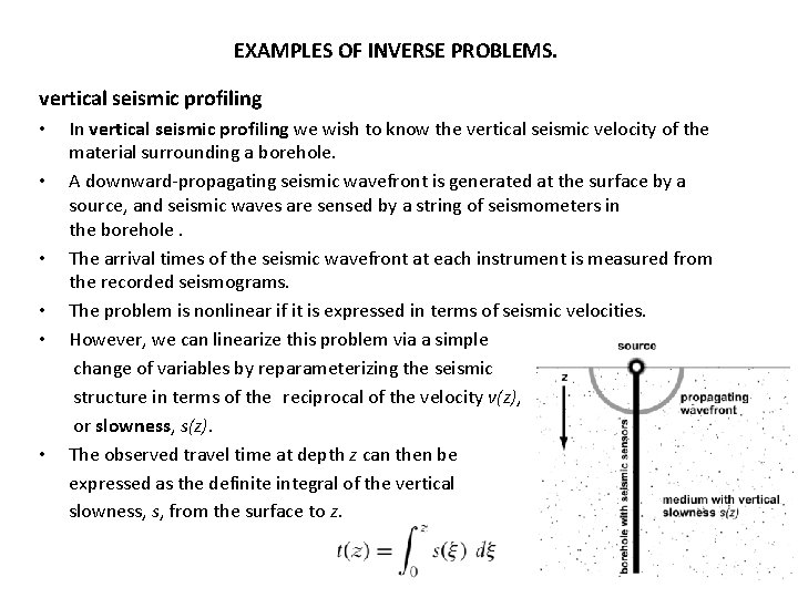
EXAMPLES OF INVERSE PROBLEMS. vertical seismic profiling • • • In vertical seismic profiling we wish to know the vertical seismic velocity of the material surrounding a borehole. A downward-propagating seismic wavefront is generated at the surface by a source, and seismic waves are sensed by a string of seismometers in the borehole. The arrival times of the seismic wavefront at each instrument is measured from the recorded seismograms. The problem is nonlinear if it is expressed in terms of seismic velocities. However, we can linearize this problem via a simple change of variables by reparameterizing the seismic structure in terms of the reciprocal of the velocity v(z), or slowness, s(z). The observed travel time at depth z can then be expressed as the definite integral of the vertical slowness, s, from the surface to z.

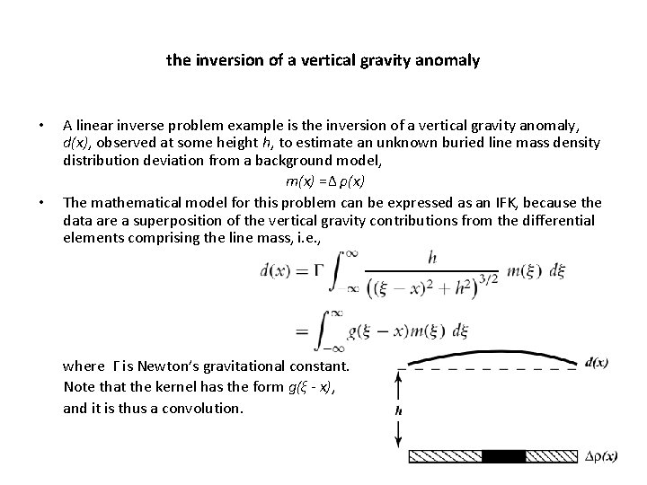
the inversion of a vertical gravity anomaly • • A linear inverse problem example is the inversion of a vertical gravity anomaly, d(x), observed at some height h, to estimate an unknown buried line mass density distribution deviation from a background model, m(x) =Δ ρ(x) The mathematical model for this problem can be expressed as an IFK, because the data are a superposition of the vertical gravity contributions from the differential elements comprising the line mass, i. e. , where Γ is Newton’s gravitational constant. Note that the kernel has the form g(ξ - x), and it is thus a convolution.

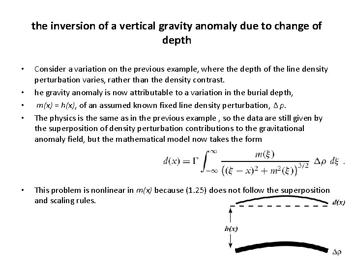
the inversion of a vertical gravity anomaly due to change of depth • • • Consider a variation on the previous example, where the depth of the line density perturbation varies, rather than the density contrast. he gravity anomaly is now attributable to a variation in the burial depth, m(x) = h(x), of an assumed known fixed line density perturbation, Δ ρ. The physics is the same as in the previous example , so the data are still given by the superposition of density perturbation contributions to the gravitational anomaly field, but the mathematical model now takes the form This problem is nonlinear in m(x) because (1. 25) does not follow the superposition and scaling rules.

cross-well tomography • • An important inverse problem is tomography, from the Greek roots tomos, “to section” or “to cut” and graphein, “to write. ” Tomography is the general technique of determining models that are consistent with path-integrated properties such as attenuation (e. g. , X-ray, radar, muon, seismic), travel time (e. g. , electromagnetic, seismic, or acoustic), or source intensity (e. g. , positron emission). One important geophysical example is cross-well tomography, where seismic sources are installed in a borehole, and the signals are received by sensors in another borehole. Another important example is joint earthquake location/velocity structure inversion carried out on scales ranging from a fraction of a cubic kilometer to global.

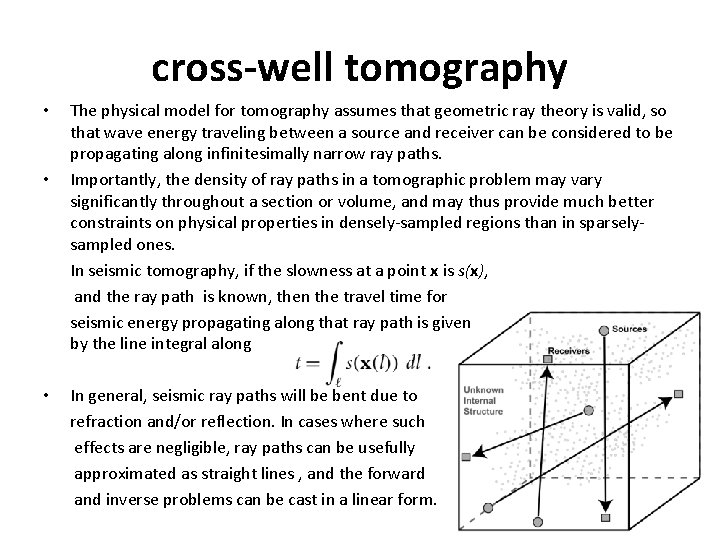
cross-well tomography • • • The physical model for tomography assumes that geometric ray theory is valid, so that wave energy traveling between a source and receiver can be considered to be propagating along infinitesimally narrow ray paths. Importantly, the density of ray paths in a tomographic problem may vary significantly throughout a section or volume, and may thus provide much better constraints on physical properties in densely-sampled regions than in sparselysampled ones. In seismic tomography, if the slowness at a point x is s(x), and the ray path is known, then the travel time for seismic energy propagating along that ray path is given by the line integral along In general, seismic ray paths will be bent due to refraction and/or reflection. In cases where such effects are negligible, ray paths can be usefully approximated as straight lines , and the forward and inverse problems can be cast in a linear form.

• However, if the ray paths are significantly bent by heterogeneous structure, the resulting inverse problem will be nonlinear.

WHY INVERSE PROBLEMS ARE HARD well-posed and ill-posed inverse problems • Essential issues that must be considered include solution existence, solution uniqueness, and instability of the solution process. 1. Existence. There may be no model that exactly fits the data. This can occur in practice because the mathematical model of the system’s physics is approximate (or perhaps simply incorrect) or because the data contain noise. 2. Uniqueness. If exact solutions do exist, they may not be unique, even for an infinite number of exact data points. That is, there may be other solutions besides mtrue that exactly satisfy G(m) = dtrue. This situation commonly occurs in potential field problems. There an infinite number of mathematically acceptable models fit to the data. 3. Instability. The process of computing an inverse solution can be extremely unstable in that a small change in measurement can lead to an enormous change in the estimated model.

WHY INVERSE PROBLEMS ARE HARD well-posed and ill-posed inverse problems • • • Inverse problems where the solution exist, is unique and stable are referred to as well-posed. On the other hand if any of these three conditions is not satisfied the inverse problems are referred to as ill-posed in the case of continuous systems, or ill-conditioned in the case of discrete linear systems. The solution of the later problems require stabilizing the solution by the use of regularization. A key point is that it is commonly possible to stabilize the inversion process by imposing additional constraints that bias the solution, a process that is generally referred to as regularization. Regularization is frequently essential to producing a usable solution to an otherwise intractable ill-posed or ill-conditioned inverse problem.