Chapter 7 Theory and Estimation of Production Managerial

Chapter 7 Theory and Estimation of Production Managerial Economics: Economic Tools for Today’s Decision Makers, 4/e By Paul Keat and Philip Young

The Theory and Estimation of Production • The Production Function • Production in the Short Run • • Total, Average, and Marginal Product Law of Diminishing Returns Stages of Production Optimal Input Usage • Production in the Long Run • Returns to Scale 2003 Prentice Hall Business Publishing Managerial Economics, 4/e Keat/Young

The Production Function • A production function defines the relationship between inputs and the maximum amount that can be produced within a given time period with a given technology. 2003 Prentice Hall Business Publishing Managerial Economics, 4/e Keat/Young

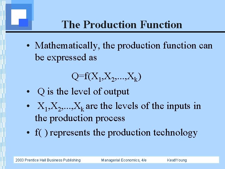
The Production Function • Mathematically, the production function can be expressed as Q=f(X 1, X 2, . . . , Xk) • Q is the level of output • X 1, X 2, . . . , Xk are the levels of the inputs in the production process • f( ) represents the production technology 2003 Prentice Hall Business Publishing Managerial Economics, 4/e Keat/Young

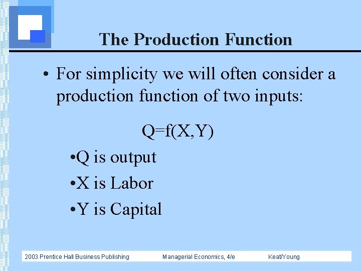
The Production Function • For simplicity we will often consider a production function of two inputs: Q=f(X, Y) • Q is output • X is Labor • Y is Capital 2003 Prentice Hall Business Publishing Managerial Economics, 4/e Keat/Young

The Production Function • When discussing production, it is important to distinguish between two time frames. • The short-run production function describes the maximum quantity of good or service that can be produced by a set of inputs, assuming that at least one of the inputs is fixed at some level. 2003 Prentice Hall Business Publishing Managerial Economics, 4/e Keat/Young

The Production Function • The long-run production function describes the maximum quantity of good or service that can be produced by a set of inputs, assuming that the firm is free to adjust the level of all inputs. 2003 Prentice Hall Business Publishing Managerial Economics, 4/e Keat/Young

Production in the Short Run • When discussing production in the short run, three definitions are important. • Total Product • Marginal Product • Average Product 2003 Prentice Hall Business Publishing Managerial Economics, 4/e Keat/Young

Production in the Short Run • Total product (TP) is another name for output in the short run. The total product function is the same as the short run production function. 2003 Prentice Hall Business Publishing Managerial Economics, 4/e Keat/Young

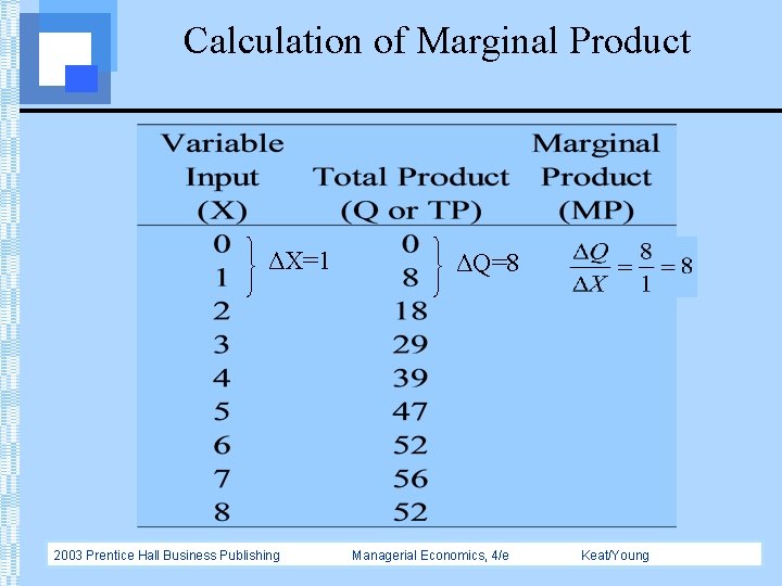
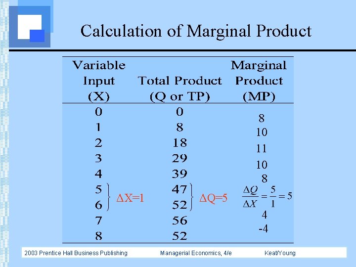
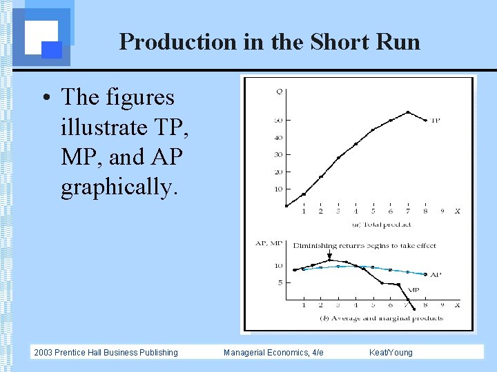
Production in the Short Run • The marginal product (MP) of a variable input is the change in output (or TP) resulting from a one unit change in the input. • MP tells us how output changes as we change the level of the input by one unit. 2003 Prentice Hall Business Publishing Managerial Economics, 4/e Keat/Young

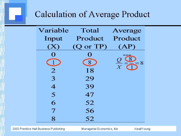
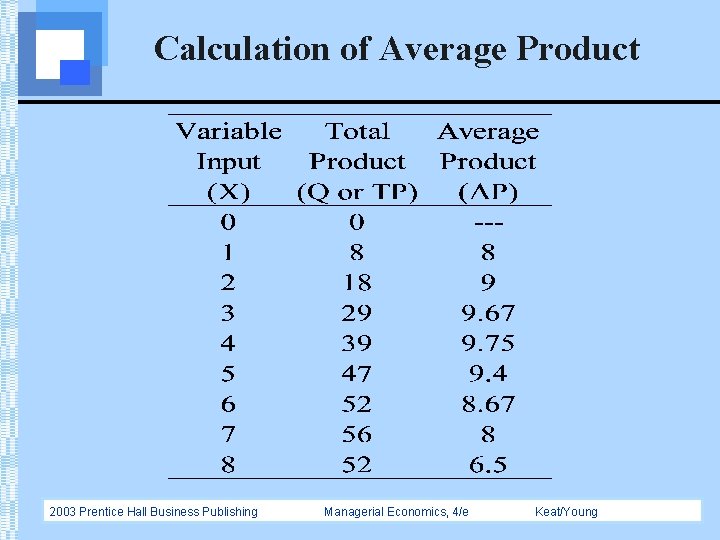
Production in the Short Run • The average product (AP) of an input is the total product divided by the level of the input. • AP tells us, on average, how many units of output are produced per unit of input used. 2003 Prentice Hall Business Publishing Managerial Economics, 4/e Keat/Young

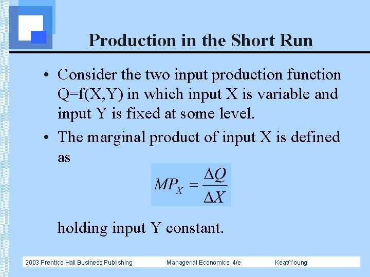
Production in the Short Run • Consider the two input production function Q=f(X, Y) in which input X is variable and input Y is fixed at some level. • The marginal product of input X is defined as holding input Y constant. 2003 Prentice Hall Business Publishing Managerial Economics, 4/e Keat/Young

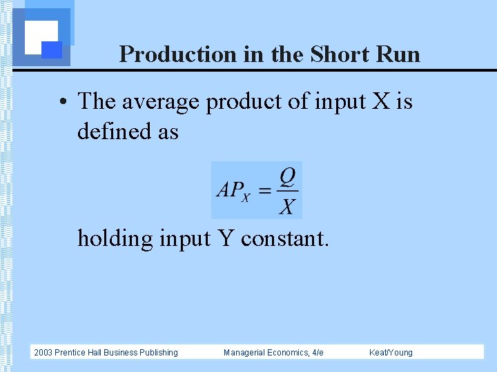
Production in the Short Run • The average product of input X is defined as holding input Y constant. 2003 Prentice Hall Business Publishing Managerial Economics, 4/e Keat/Young

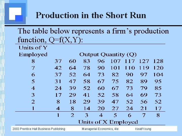
Production in the Short Run The table below represents a firm’s production function, Q=f(X, Y): 2003 Prentice Hall Business Publishing Managerial Economics, 4/e Keat/Young

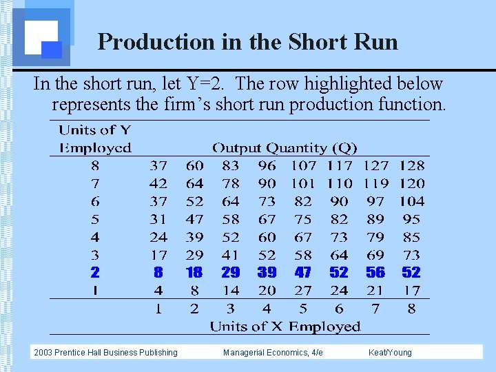
Production in the Short Run In the short run, let Y=2. The row highlighted below represents the firm’s short run production function. 2003 Prentice Hall Business Publishing Managerial Economics, 4/e Keat/Young

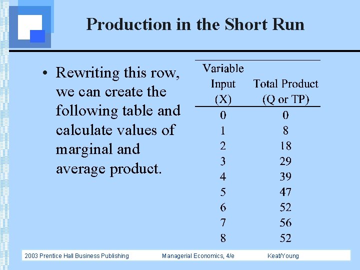
Production in the Short Run • Rewriting this row, we can create the following table and calculate values of marginal and average product. 2003 Prentice Hall Business Publishing Managerial Economics, 4/e Keat/Young

Calculation of Marginal Product ΔX=1 2003 Prentice Hall Business Publishing ΔQ=8 Managerial Economics, 4/e Keat/Young

Calculation of Marginal Product 8 10 11 10 8 ΔX=1 ΔQ=5 4 -4 2003 Prentice Hall Business Publishing Managerial Economics, 4/e Keat/Young

Calculation of Average Product 1 2003 Prentice Hall Business Publishing 8 Managerial Economics, 4/e 8 1 Keat/Young

Calculation of Average Product 2003 Prentice Hall Business Publishing Managerial Economics, 4/e Keat/Young

Production in the Short Run • The figures illustrate TP, MP, and AP graphically. 2003 Prentice Hall Business Publishing Managerial Economics, 4/e Keat/Young

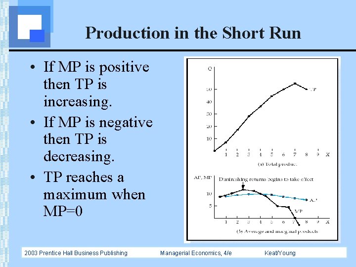
Production in the Short Run • If MP is positive then TP is increasing. • If MP is negative then TP is decreasing. • TP reaches a maximum when MP=0 2003 Prentice Hall Business Publishing Managerial Economics, 4/e Keat/Young

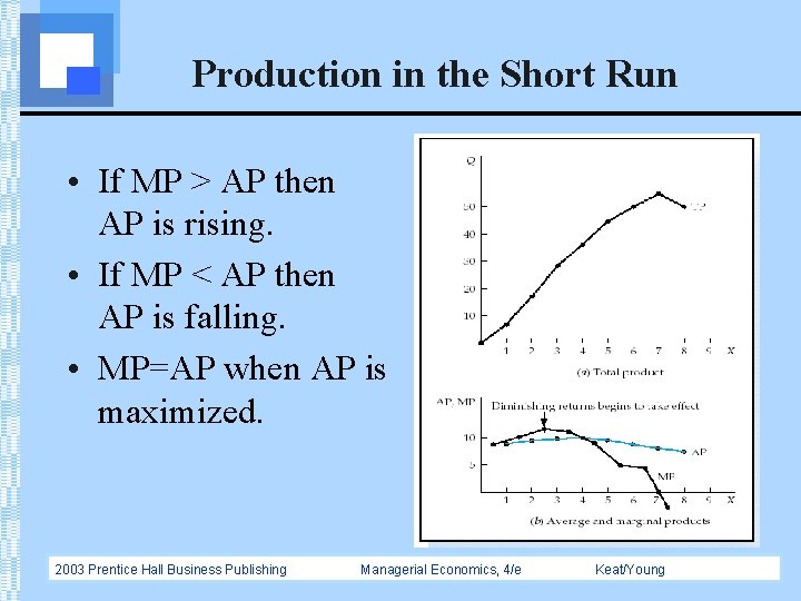
Production in the Short Run • If MP > AP then AP is rising. • If MP < AP then AP is falling. • MP=AP when AP is maximized. 2003 Prentice Hall Business Publishing Managerial Economics, 4/e Keat/Young

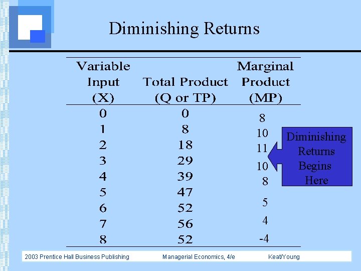
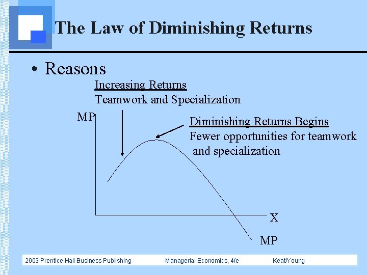
The Law of Diminishing Returns • Definition • As additional units of a variable input are combined with a fixed input, at some point the additional output (i. e. , marginal product) starts to diminish. 2003 Prentice Hall Business Publishing Managerial Economics, 4/e Keat/Young

Diminishing Returns 8 10 11 10 8 Diminishing Returns Begins Here 5 4 -4 2003 Prentice Hall Business Publishing Managerial Economics, 4/e Keat/Young

The Law of Diminishing Returns • Reasons Increasing Returns Teamwork and Specialization MP Diminishing Returns Begins Fewer opportunities for teamwork and specialization X MP 2003 Prentice Hall Business Publishing Managerial Economics, 4/e Keat/Young

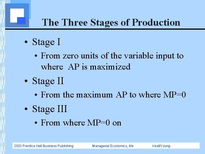
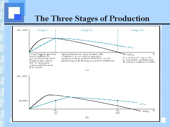
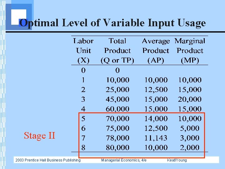
The Three Stages of Production • Stage I • From zero units of the variable input to where AP is maximized • Stage II • From the maximum AP to where MP=0 • Stage III • From where MP=0 on 2003 Prentice Hall Business Publishing Managerial Economics, 4/e Keat/Young

The Three Stages of Production 2003 Prentice Hall Business Publishing Managerial Economics, 4/e Keat/Young

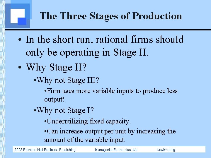
The Three Stages of Production • In the short run, rational firms should only be operating in Stage II. • Why Stage II? • Why not Stage III? • Firm uses more variable inputs to produce less output! • Why not Stage I? • Underutilizing fixed capacity. • Can increase output per unit by increasing the amount of the variable input. 2003 Prentice Hall Business Publishing Managerial Economics, 4/e Keat/Young

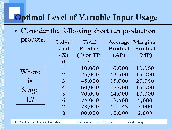
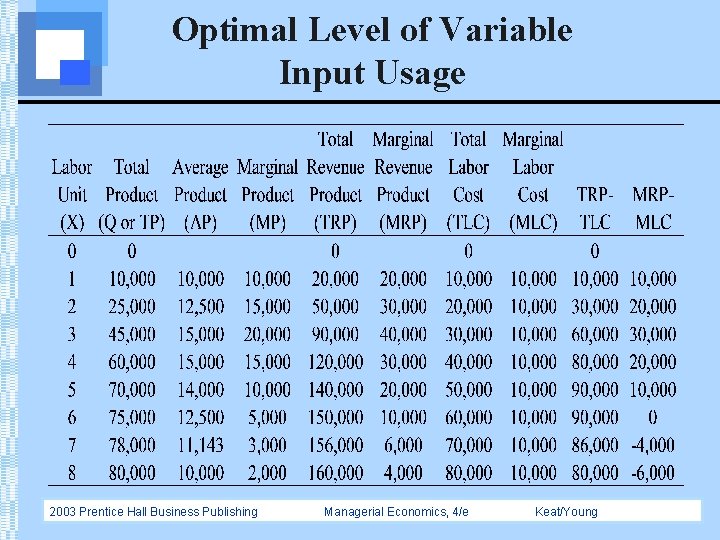
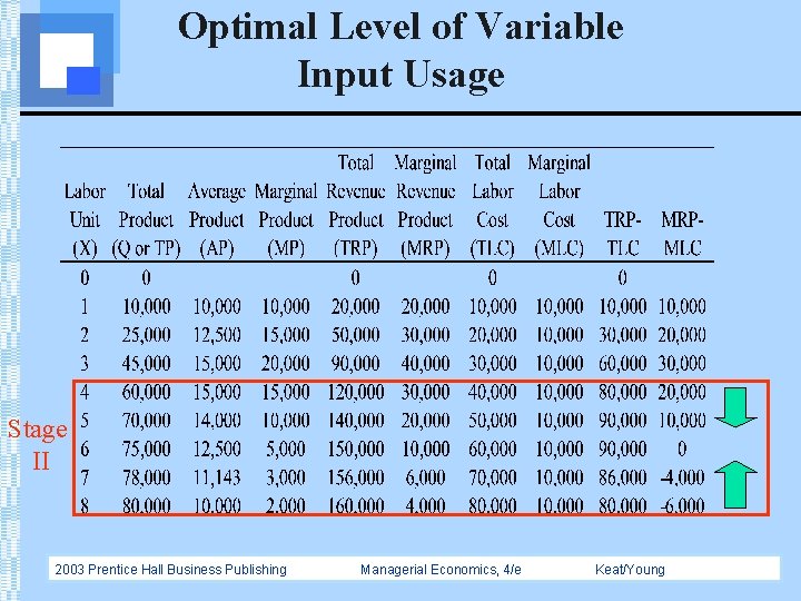
Optimal Level of Variable Input Usage • Consider the following short run production process. Where is Stage II? 2003 Prentice Hall Business Publishing Managerial Economics, 4/e Keat/Young

Optimal Level of Variable Input Usage Stage II 2003 Prentice Hall Business Publishing Managerial Economics, 4/e Keat/Young

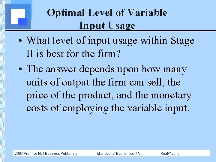
Optimal Level of Variable Input Usage • What level of input usage within Stage II is best for the firm? • The answer depends upon how many units of output the firm can sell, the price of the product, and the monetary costs of employing the variable input. 2003 Prentice Hall Business Publishing Managerial Economics, 4/e Keat/Young

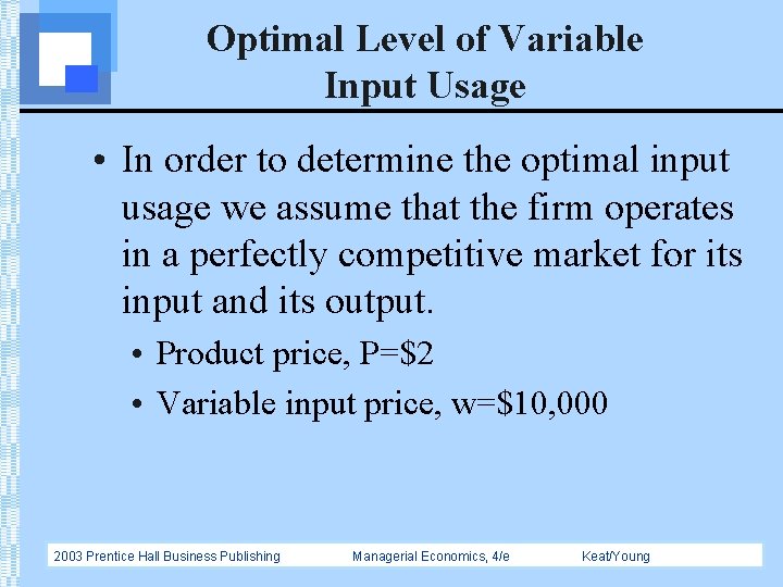
Optimal Level of Variable Input Usage • In order to determine the optimal input usage we assume that the firm operates in a perfectly competitive market for its input and its output. • Product price, P=$2 • Variable input price, w=$10, 000 2003 Prentice Hall Business Publishing Managerial Economics, 4/e Keat/Young

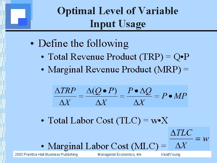
Optimal Level of Variable Input Usage • Define the following • Total Revenue Product (TRP) = Q • P • Marginal Revenue Product (MRP) = • Total Labor Cost (TLC) = w • X • Marginal Labor Cost (MLC) = 2003 Prentice Hall Business Publishing Managerial Economics, 4/e Keat/Young

Optimal Level of Variable Input Usage 2003 Prentice Hall Business Publishing Managerial Economics, 4/e Keat/Young

Optimal Level of Variable Input Usage Stage II 2003 Prentice Hall Business Publishing Managerial Economics, 4/e Keat/Young

Optimal Level of Variable Input Usage • A profit-maximizing firm operating in perfectly competitive output and input markets will be using the optimal amount of an input at the point at which the monetary value of the input’s marginal product is equal to the additional cost of using that input. • Where MRP=MLC. 2003 Prentice Hall Business Publishing Managerial Economics, 4/e Keat/Young

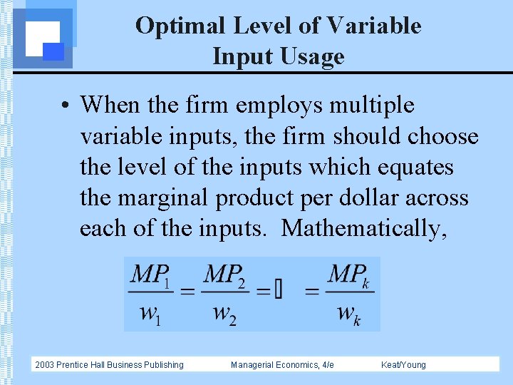
Optimal Level of Variable Input Usage • When the firm employs multiple variable inputs, the firm should choose the level of the inputs which equates the marginal product per dollar across each of the inputs. Mathematically, 2003 Prentice Hall Business Publishing Managerial Economics, 4/e Keat/Young

Production in the Long Run • In the long run, all inputs are variable. • The long run production process is described by the concept of returns to scale. • Returns to scale describes what happens to total output as all of the inputs are changed by the same proportion. 2003 Prentice Hall Business Publishing Managerial Economics, 4/e Keat/Young

Production in the Long Run • If all inputs into the production process are doubled, three things can happen: • output can more than double • increasing returns to scale (IRTS) • output can exactly double • constant returns to scale (CRTS) • output can less than double • decreasing returns to scale (DRTS) 2003 Prentice Hall Business Publishing Managerial Economics, 4/e Keat/Young

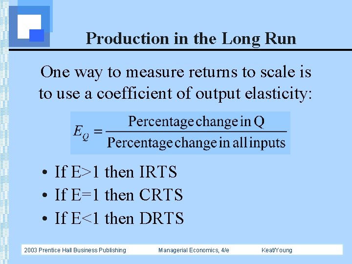
Production in the Long Run One way to measure returns to scale is to use a coefficient of output elasticity: • If E>1 then IRTS • If E=1 then CRTS • If E<1 then DRTS 2003 Prentice Hall Business Publishing Managerial Economics, 4/e Keat/Young

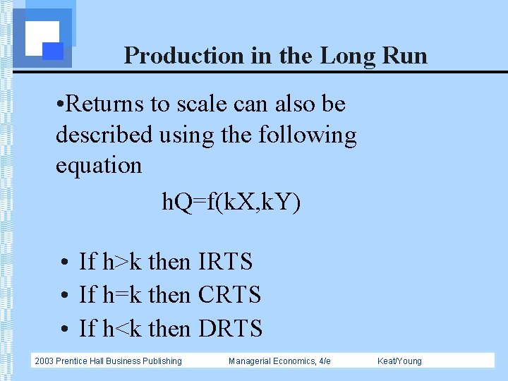
Production in the Long Run • Returns to scale can also be described using the following equation h. Q=f(k. X, k. Y) • If h>k then IRTS • If h=k then CRTS • If h<k then DRTS 2003 Prentice Hall Business Publishing Managerial Economics, 4/e Keat/Young

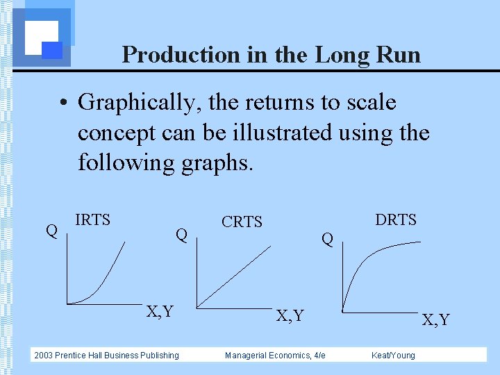
Production in the Long Run • Graphically, the returns to scale concept can be illustrated using the following graphs. Q IRTS Q X, Y 2003 Prentice Hall Business Publishing DRTS CRTS Q X, Y Managerial Economics, 4/e X, Y Keat/Young

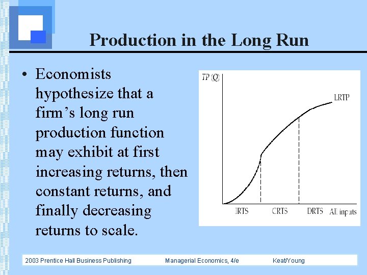
Production in the Long Run • Economists hypothesize that a firm’s long run production function may exhibit at first increasing returns, then constant returns, and finally decreasing returns to scale. 2003 Prentice Hall Business Publishing Managerial Economics, 4/e Keat/Young