Chapter 5 Demand Estimation and Forecasting Chapter Outline

Chapter 5 Demand Estimation and Forecasting

Chapter Outline • • • Regression analysis Limitation of regression analysis The importance of business forecasting Prerequisites of a good forecast Forecasting techniques Copyright © 2014 Pearson Education, Inc. All rights reserved. 5 -2

Learning Objectives • Understand the importance of forecasting in business • Know how to specify and interpret a regression model • Describe the major forecasting techniques used in business and their limitations • Explain basic smoothing methods of forecasting, such as the moving average and exponential smoothing Copyright © 2014 Pearson Education, Inc. All rights reserved. 5 -3

Data Collection • Statistical analyses are only as good as the accuracy and appropriateness of the sample of information that is used. • Several sources of data for business analysis: – buy from data providers (e. g. ACNielsen, IRI) – perform a consumer survey – focus groups – technology: point-of-sale data sources Copyright © 2014 Pearson Education, Inc. All rights reserved. 5 -4

Regression Analysis • Regression analysis: a procedure commonly used by economists to estimate consumer demand with available data Two types of regression: – cross-sectional: analyze several variables for a single period of time – time series data: analyze a single variable over multiple periods of time Copyright © 2014 Pearson Education, Inc. All rights reserved. 5 -5

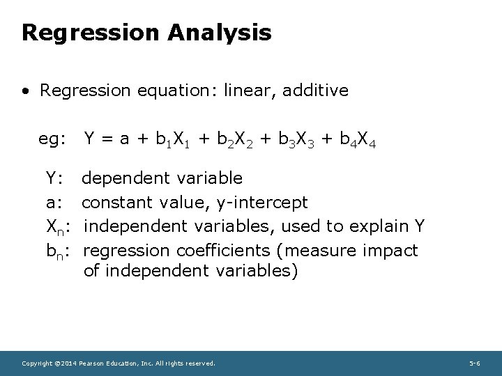
Regression Analysis • Regression equation: linear, additive eg: Y: a: Xn : bn : Y = a + b 1 X 1 + b 2 X 2 + b 3 X 3 + b 4 X 4 dependent variable constant value, y-intercept independent variables, used to explain Y regression coefficients (measure impact of independent variables) Copyright © 2014 Pearson Education, Inc. All rights reserved. 5 -6

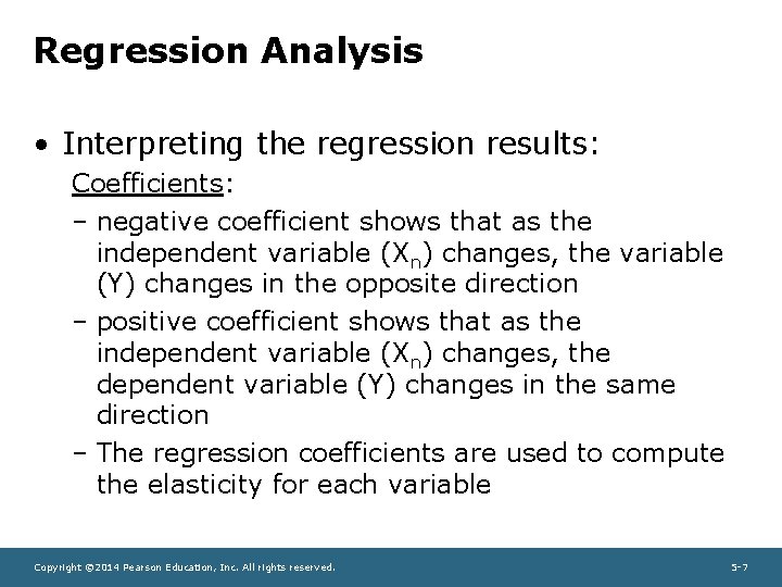
Regression Analysis • Interpreting the regression results: Coefficients: – negative coefficient shows that as the independent variable (Xn) changes, the variable (Y) changes in the opposite direction – positive coefficient shows that as the independent variable (Xn) changes, the dependent variable (Y) changes in the same direction – The regression coefficients are used to compute the elasticity for each variable Copyright © 2014 Pearson Education, Inc. All rights reserved. 5 -7

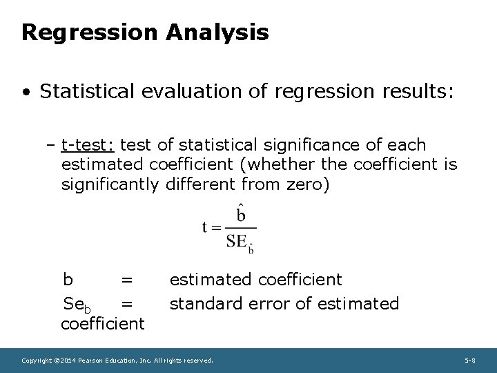
Regression Analysis • Statistical evaluation of regression results: – t-test: test of statistical significance of each estimated coefficient (whether the coefficient is significantly different from zero) b = Seb = coefficient estimated coefficient standard error of estimated Copyright © 2014 Pearson Education, Inc. All rights reserved. 5 -8

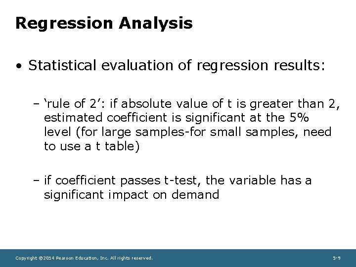
Regression Analysis • Statistical evaluation of regression results: – ‘rule of 2’: if absolute value of t is greater than 2, estimated coefficient is significant at the 5% level (for large samples-for small samples, need to use a t table) – if coefficient passes t-test, the variable has a significant impact on demand Copyright © 2014 Pearson Education, Inc. All rights reserved. 5 -9

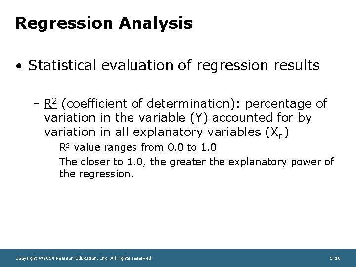
Regression Analysis • Statistical evaluation of regression results – R 2 (coefficient of determination): percentage of variation in the variable (Y) accounted for by variation in all explanatory variables (Xn) R 2 value ranges from 0. 0 to 1. 0 The closer to 1. 0, the greater the explanatory power of the regression. Copyright © 2014 Pearson Education, Inc. All rights reserved. 5 -10

Regression Analysis • Statistical evaluation of regression results – F-test: measures statistical significance of the entire regression as a whole (not each coefficient) Copyright © 2014 Pearson Education, Inc. All rights reserved. 5 -11

Regression Analysis • Steps for analyzing regression results – check coefficient signs and magnitudes – compute elasticity coefficient – determine statistical significance Copyright © 2014 Pearson Education, Inc. All rights reserved. 5 -12

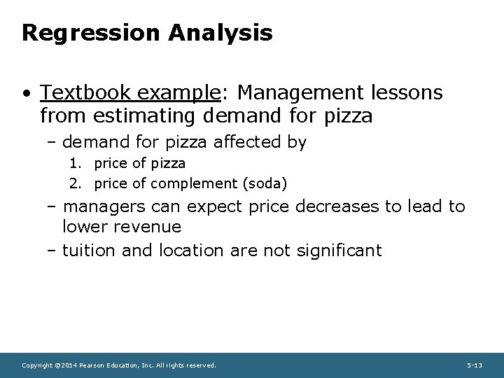
Regression Analysis • Textbook example: Management lessons from estimating demand for pizza – demand for pizza affected by 1. price of pizza 2. price of complement (soda) – managers can expect price decreases to lead to lower revenue – tuition and location are not significant Copyright © 2014 Pearson Education, Inc. All rights reserved. 5 -13

Regression Analysis • Challenges – Identification – Multicollinearity – Autocorrelation Copyright © 2014 Pearson Education, Inc. All rights reserved. 5 -14

Regression Analysis • Challenge 1: Identification problem: – The estimation of demand may produce biased results due to simultaneous shifting of supply and demand curves. – Solution: use of advanced correction techniques, such as two-stage least squares and indirect least squares may compensate for the bias Copyright © 2014 Pearson Education, Inc. All rights reserved. 5 -15

Regression Analysis • Challenge 2: Multicollinearity problem – Two or more independent variables are highly correlated, thus it is difficult to separate the effect each has on the dependent variable. – Solution: a standard remedy is to drop one of the closely related independent variables from the regression Copyright © 2014 Pearson Education, Inc. All rights reserved. 5 -16

Regression Analysis • Challenge 3: Autocorrelation problem – Also known as serial correlation, occurs when the dependent variable relates to the Y variable according to a certain pattern – Note: possible causes include omitted variables, or non-linearity; Durbin-Watson statistic is used to identify autocorrelation – Solution: to correct autocorrelation consider transforming the data into a different order of magnitude or introducing leading or lagging data Copyright © 2014 Pearson Education, Inc. All rights reserved. 5 -17

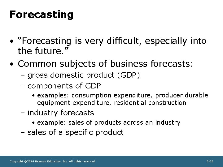
Forecasting • “Forecasting is very difficult, especially into the future. ” • Common subjects of business forecasts: – gross domestic product (GDP) – components of GDP • examples: consumption expenditure, producer durable equipment expenditure, residential construction – industry forecasts • example: sales of products across an industry – sales of a specific product Copyright © 2014 Pearson Education, Inc. All rights reserved. 5 -18

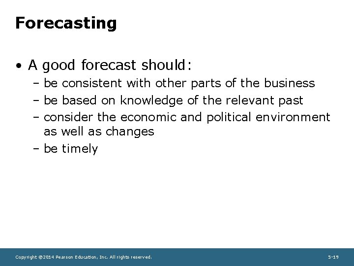
Forecasting • A good forecast should: – be consistent with other parts of the business – be based on knowledge of the relevant past – consider the economic and political environment as well as changes – be timely Copyright © 2014 Pearson Education, Inc. All rights reserved. 5 -19

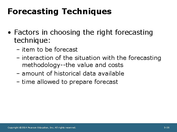
Forecasting Techniques • Factors in choosing the right forecasting technique: – item to be forecast – interaction of the situation with the forecasting methodology--the value and costs – amount of historical data available – time allowed to prepare forecast Copyright © 2014 Pearson Education, Inc. All rights reserved. 5 -20

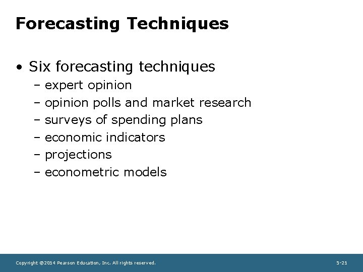
Forecasting Techniques • Six forecasting techniques – expert opinion – opinion polls and market research – surveys of spending plans – economic indicators – projections – econometric models Copyright © 2014 Pearson Education, Inc. All rights reserved. 5 -21

Forecasting Techniques • Approaches to forecasting – qualitative forecasting is based on judgments expressed by individuals or group – quantitative forecasting utilizes significant amounts of data and equations Copyright © 2014 Pearson Education, Inc. All rights reserved. 5 -22

Forecasting Techniques • Approaches to quantitative forecasting: – naïve forecasting projects past data without explaining future trends – causal (or explanatory) forecasting attempts to explain the functional relationships between the dependent variable and the independent variables Copyright © 2014 Pearson Education, Inc. All rights reserved. 5 -23

Forecasting Techniques • Expert opinion techniques – Jury of executive opinion: forecasts generated by a group of corporate executives assembled together Copyright © 2014 Pearson Education, Inc. All rights reserved. 5 -24

Forecasting Techniques • Expert opinion techniques – The Delphi method: a form of expert opinion forecasting that uses a series of questions and answers to obtain a consensus forecast, where experts do not meet Copyright © 2014 Pearson Education, Inc. All rights reserved. 5 -25

Forecasting Techniques • Opinion polls: sample populations are surveyed to determine consumption trends – may identify changes in trends – choice of sample is important – questions must be simple and clear Copyright © 2014 Pearson Education, Inc. All rights reserved. 5 -26

Forecasting Techniques • Market research: is closely related to opinion polling and will indicate not only why the consumer is (or is not) buying, but also – who the consumer is – how he or she is using the product – characteristics the consumer thinks are most important in the purchasing decision Copyright © 2014 Pearson Education, Inc. All rights reserved. 5 -27

Forecasting Techniques • Surveys of spending plans: yields information about ‘macro-type’ data relating to the economy, especially: – consumer intentions • examples: Survey of Consumers (University of Michigan), Consumer Confidence Survey (Conference Board) – inventories and sales expectations Copyright © 2014 Pearson Education, Inc. All rights reserved. 5 -28

Forecasting Techniques • Economic indicators: a barometric method of forecasting designed to alert business to changes in conditions – leading, coincident, and lagging indicators – composite index: one indicator alone may not be very reliable, but a mix of leading indicators may be effective Copyright © 2014 Pearson Education, Inc. All rights reserved. 5 -29

Forecasting Techniques • Leading indicators predict future economic activity – average hours, manufacturing – initial claims for unemployment insurance – manufacturers’ new orders for consumer goods and materials – vendor performance, slower deliveries diffusion index – manufacturers’ new orders, nondefense capital goods Copyright © 2014 Pearson Education, Inc. All rights reserved. 5 -30

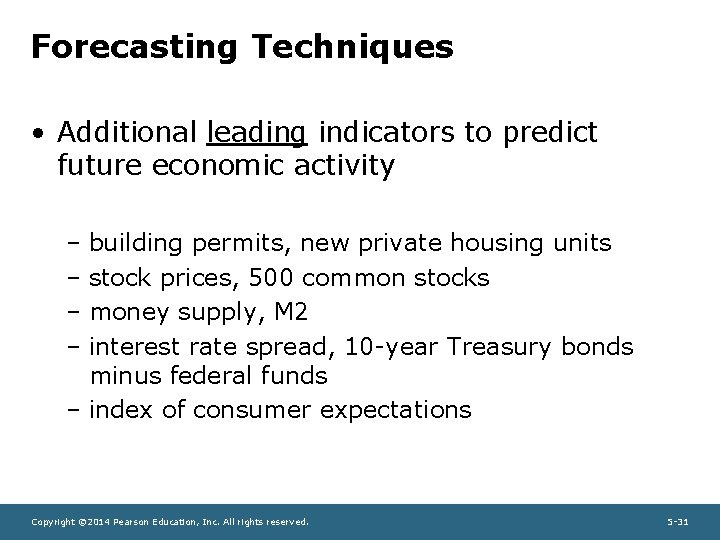
Forecasting Techniques • Additional leading indicators to predict future economic activity – building permits, new private housing units – stock prices, 500 common stocks – money supply, M 2 – interest rate spread, 10 -year Treasury bonds minus federal funds – index of consumer expectations Copyright © 2014 Pearson Education, Inc. All rights reserved. 5 -31

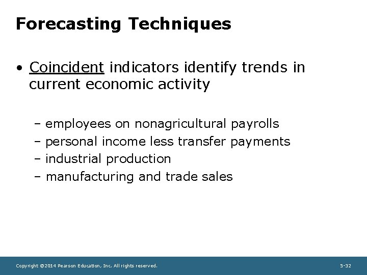
Forecasting Techniques • Coincident indicators identify trends in current economic activity – employees on nonagricultural payrolls – personal income less transfer payments – industrial production – manufacturing and trade sales Copyright © 2014 Pearson Education, Inc. All rights reserved. 5 -32

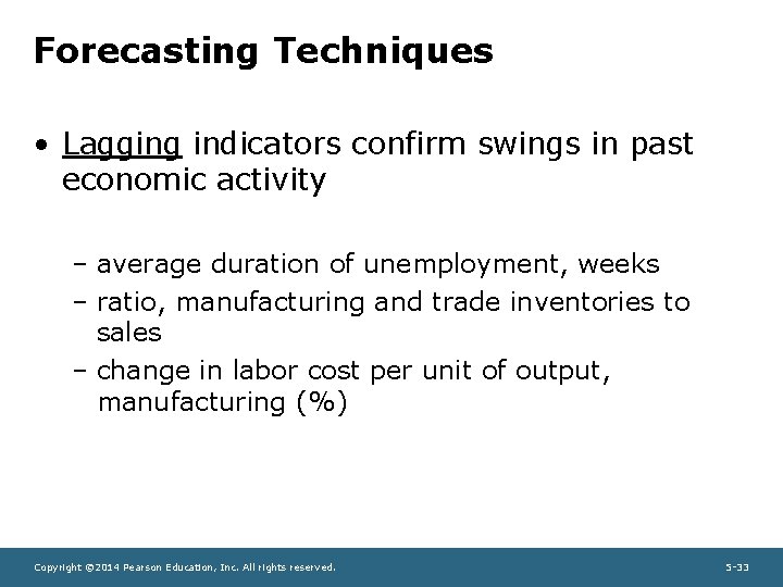
Forecasting Techniques • Lagging indicators confirm swings in past economic activity – average duration of unemployment, weeks – ratio, manufacturing and trade inventories to sales – change in labor cost per unit of output, manufacturing (%) Copyright © 2014 Pearson Education, Inc. All rights reserved. 5 -33

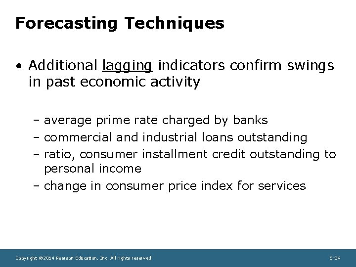
Forecasting Techniques • Additional lagging indicators confirm swings in past economic activity – average prime rate charged by banks – commercial and industrial loans outstanding – ratio, consumer installment credit outstanding to personal income – change in consumer price index for services Copyright © 2014 Pearson Education, Inc. All rights reserved. 5 -34

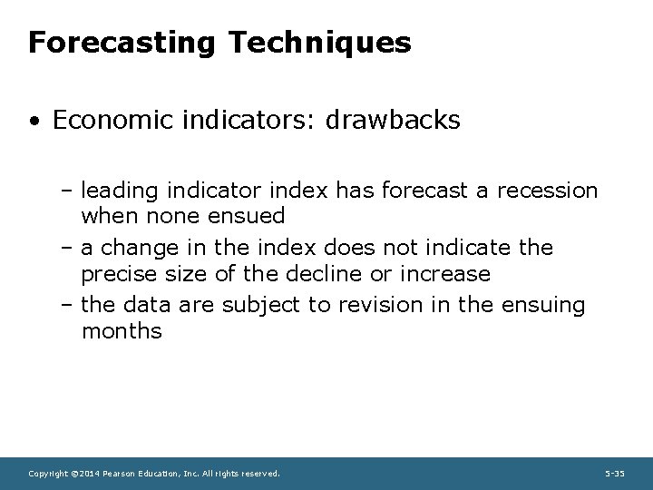
Forecasting Techniques • Economic indicators: drawbacks – leading indicator index has forecast a recession when none ensued – a change in the index does not indicate the precise size of the decline or increase – the data are subject to revision in the ensuing months Copyright © 2014 Pearson Education, Inc. All rights reserved. 5 -35

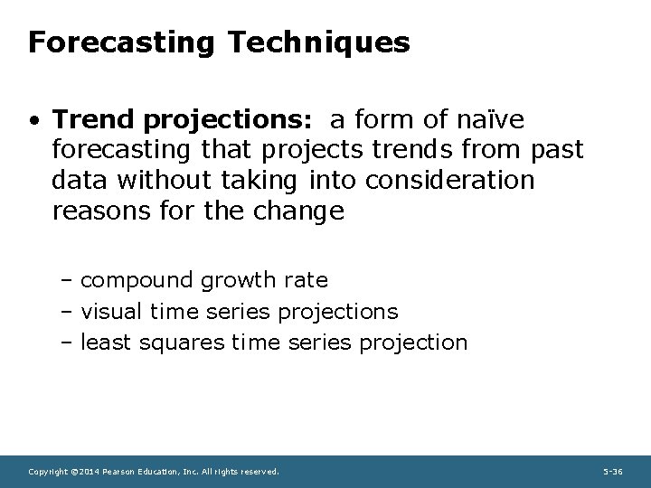
Forecasting Techniques • Trend projections: a form of naïve forecasting that projects trends from past data without taking into consideration reasons for the change – compound growth rate – visual time series projections – least squares time series projection Copyright © 2014 Pearson Education, Inc. All rights reserved. 5 -36

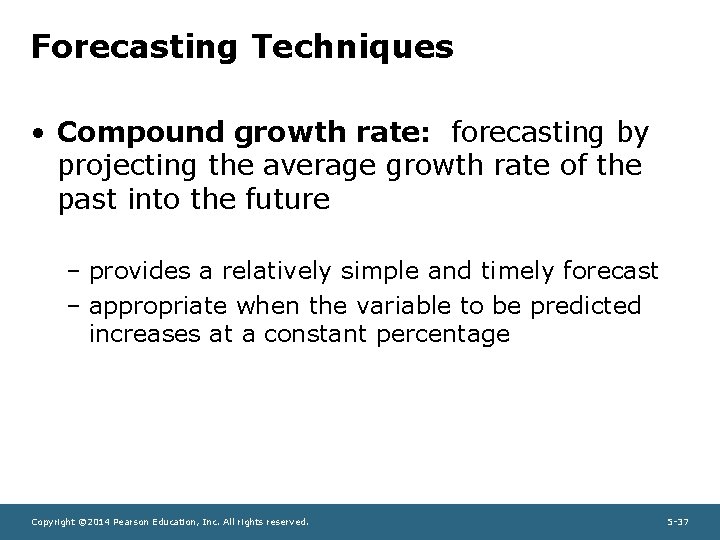
Forecasting Techniques • Compound growth rate: forecasting by projecting the average growth rate of the past into the future – provides a relatively simple and timely forecast – appropriate when the variable to be predicted increases at a constant percentage Copyright © 2014 Pearson Education, Inc. All rights reserved. 5 -37

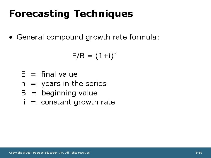
Forecasting Techniques • General compound growth rate formula: E/B = (1+i)n E n B i = = final value years in the series beginning value constant growth rate Copyright © 2014 Pearson Education, Inc. All rights reserved. 5 -38

Forecasting Techniques • Visual time series projections: plotting observations on a graph and viewing the shape of the data and any trends Copyright © 2014 Pearson Education, Inc. All rights reserved. 5 -39

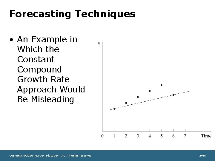
Forecasting Techniques • An Example in Which the Constant Compound Growth Rate Approach Would Be Misleading Copyright © 2014 Pearson Education, Inc. All rights reserved. 5 -40

Forecasting Techniques • Time series analysis: a naïve method of forecasting from past data by using least squares statistical methods to identify trends, cycles, seasonality, and irregular movements Copyright © 2014 Pearson Education, Inc. All rights reserved. 5 -41

Forecasting Techniques • Time series analysis: – easy to calculate – does not require much judgment or analytical skill – describes the best possible fit for past data – usually reasonably reliable in the short run Copyright © 2014 Pearson Education, Inc. All rights reserved. 5 -42

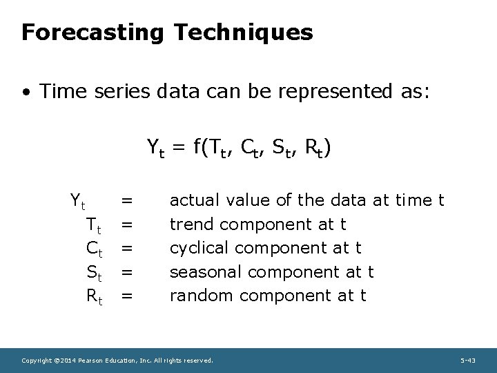
Forecasting Techniques • Time series data can be represented as: Yt = f(Tt, Ct, St, Rt) Yt Tt Ct St Rt = = = actual value of the data at time t trend component at t cyclical component at t seasonal component at t random component at t Copyright © 2014 Pearson Education, Inc. All rights reserved. 5 -43

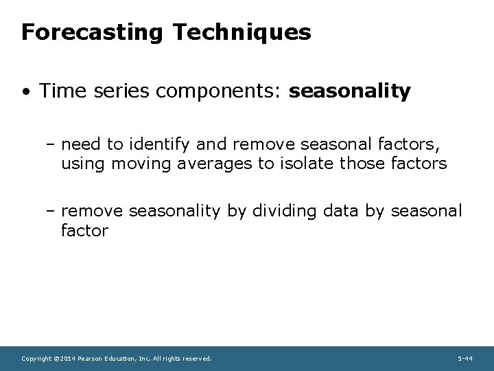
Forecasting Techniques • Time series components: seasonality – need to identify and remove seasonal factors, using moving averages to isolate those factors – remove seasonality by dividing data by seasonal factor Copyright © 2014 Pearson Education, Inc. All rights reserved. 5 -44

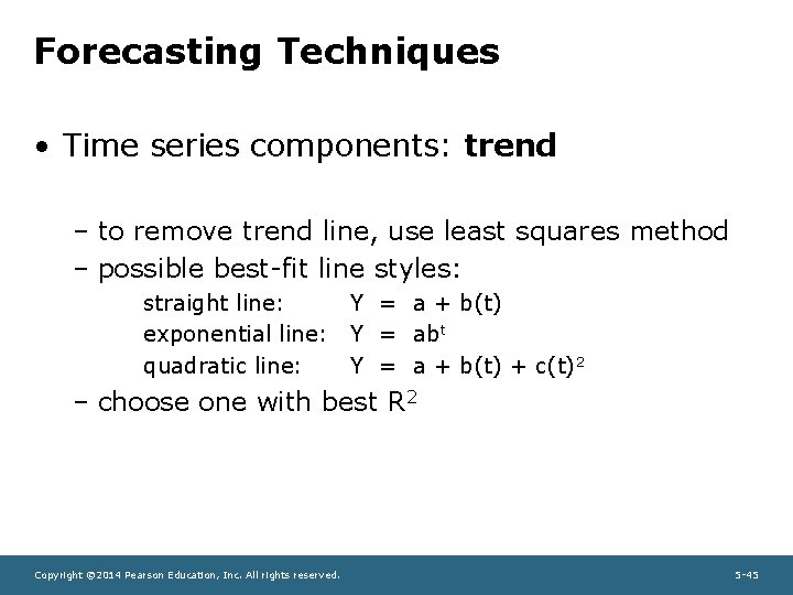
Forecasting Techniques • Time series components: trend – to remove trend line, use least squares method – possible best-fit line styles: straight line: exponential line: quadratic line: Y = a + b(t) Y = abt Y = a + b(t) + c(t)2 – choose one with best R 2 Copyright © 2014 Pearson Education, Inc. All rights reserved. 5 -45

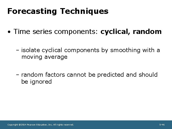
Forecasting Techniques • Time series components: cyclical, random – isolate cyclical components by smoothing with a moving average – random factors cannot be predicted and should be ignored Copyright © 2014 Pearson Education, Inc. All rights reserved. 5 -46

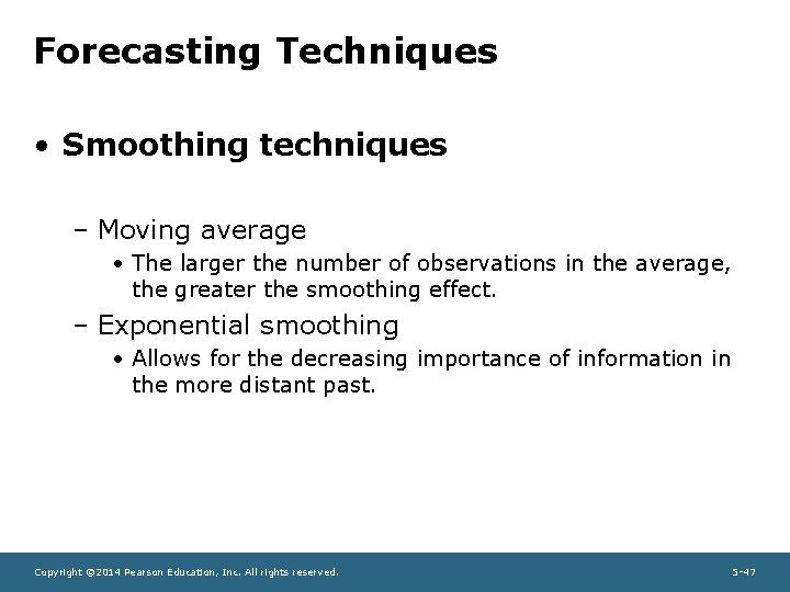
Forecasting Techniques • Smoothing techniques – Moving average • The larger the number of observations in the average, the greater the smoothing effect. – Exponential smoothing • Allows for the decreasing importance of information in the more distant past. Copyright © 2014 Pearson Education, Inc. All rights reserved. 5 -47

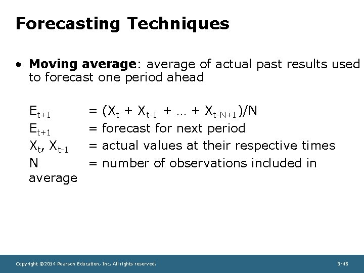
Forecasting Techniques • Moving average: average of actual past results used to forecast one period ahead Et+1 Xt, Xt-1 N average = = (Xt + Xt-1 + … + Xt-N+1)/N forecast for next period actual values at their respective times number of observations included in Copyright © 2014 Pearson Education, Inc. All rights reserved. 5 -48

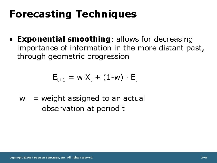
Forecasting Techniques • Exponential smoothing: allows for decreasing importance of information in the more distant past, through geometric progression Et+1 = w·Xt + (1 -w) · Et w = weight assigned to an actual observation at period t Copyright © 2014 Pearson Education, Inc. All rights reserved. 5 -49

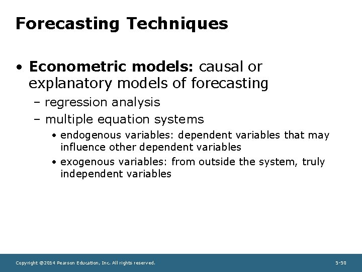
Forecasting Techniques • Econometric models: causal or explanatory models of forecasting – regression analysis – multiple equation systems • endogenous variables: dependent variables that may influence other dependent variables • exogenous variables: from outside the system, truly independent variables Copyright © 2014 Pearson Education, Inc. All rights reserved. 5 -50

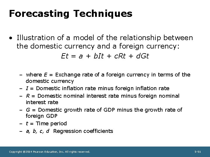
Forecasting Techniques • Illustration of a model of the relationship between the domestic currency and a foreign currency: Et = a + b. It + c. Rt + d. Gt – where E = Exchange rate of a foreign currency in terms of the domestic currency – I = Domestic inflation rate minus foreign inflation rate – R = Domestic nominal interest rate minus foreign nominal interest rate – G = Domestic growth rate of GDP minus the growth rate of foreign GDP – t = Time period – a, b, c, d Regression coefficients Copyright © 2014 Pearson Education, Inc. All rights reserved. 5 -51

Summary • Regression analysis is a primary tool used by businesses to understand demand. • Reliable input data and proper estimation and evaluation are needed. • Forecasting is an important activity in many organizations. In business, forecasting is a necessity. • This chapter summarized and discussed six of the major forecasting techniques used by businesses. Copyright © 2014 Pearson Education, Inc. All rights reserved. 5 -52