BEC 30325 Managerial Economics Theory of Production Cost

BEC 30325 Managerial Economics Theory of Production & Cost

Fundamental questions… • How can production be optimized? • How can cost be minimized? • How does output behave when quantity of inputs is increased? • How can the least-cost combination of inputs be achieved? • What does happen to the rate of return when more plants are added? • How does technology matter in reducing the cost of production? 2

Why production and cost? ? ? • Profit through managing the revenue is more interesting and exciting. • Managers may enjoy time spent on revenue decisions. • In a competitive market scenario; – Profitability fairly depends on optimization of production and minimization of costs. – Managers may find internalization of profitability is easier than externalization. 3

Some basic concepts of production theory… • Fixed and variable inputs – Fixed inputs (Ex: buildings, machinery) • Economic sense – supply is inelastic in the short run • Technical sense – remains constant for a certain level of output • Quasi-fixed inputs - unlike the fixed inputs, this can be avoided and cost is zero if the firm chooses to produce nothing – Variable inputs (Ex: raw materials, labour, fuel) • Economic sense – supply is elastic in the short run • Technical sense – changes with the change in output 4

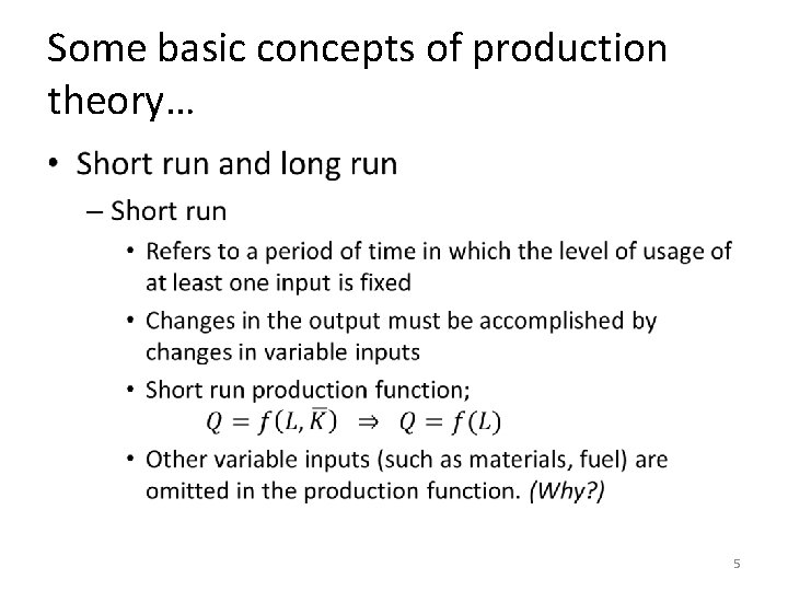
Some basic concepts of production theory… • 5

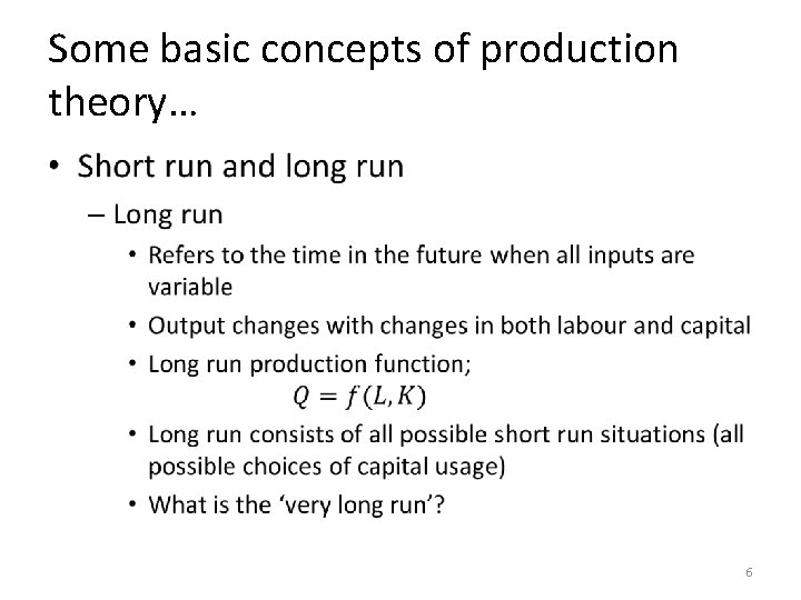
Some basic concepts of production theory… • 6

Some basic concepts of production theory… • Technical and economic efficiency – Technical efficiency • Production of the maximum level of output that can be obtained from a given combination of inputs – Economic efficiency • Production of a given amount of output at the lowest possible cost 7

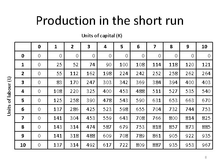
Production in the short run Units of capital (K) Units of labour (L) 0 1 2 3 4 5 6 7 8 9 10 0 0 0 1 0 25 52 74 90 108 114 118 120 121 2 0 55 112 162 198 224 242 258 262 264 3 0 83 170 247 303 342 369 384 394 400 403 4 0 108 220 325 400 453 488 511 527 535 540 5 0 125 258 390 478 543 590 631 653 663 670 6 0 137 286 425 523 598 655 704 732 744 753 7 0 141 304 453 559 643 708 766 800 814 825 8 0 143 314 474 587 679 753 818 857 873 885 9 0 141 318 488 609 708 789 861 905 922 935 10 0 137 314 492 617 722 809 887 935 953 967 8

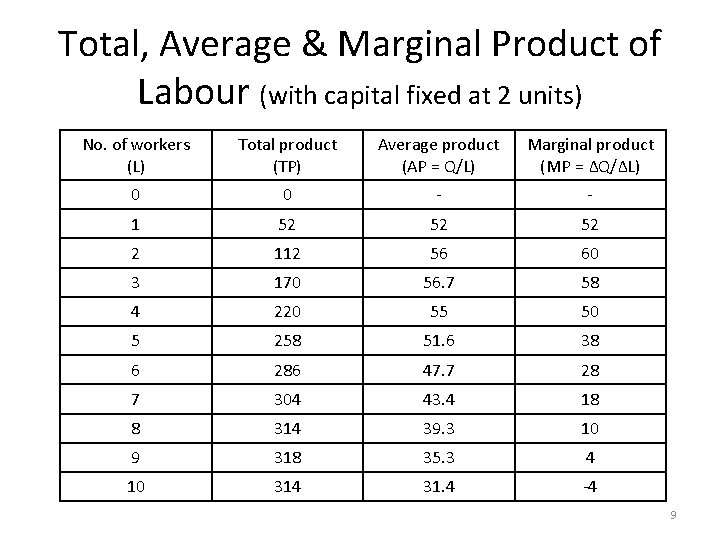
Total, Average & Marginal Product of Labour (with capital fixed at 2 units) No. of workers (L) Total product (TP) Average product (AP = Q/L) Marginal product (MP = ∆Q/∆L) 0 0 - - 1 52 52 52 2 112 56 60 3 170 56. 7 58 4 220 55 50 5 258 51. 6 38 6 286 47. 7 28 7 304 43. 4 18 8 314 39. 3 10 9 318 35. 3 4 10 314 31. 4 -4 9

Average & Marginal Products 10

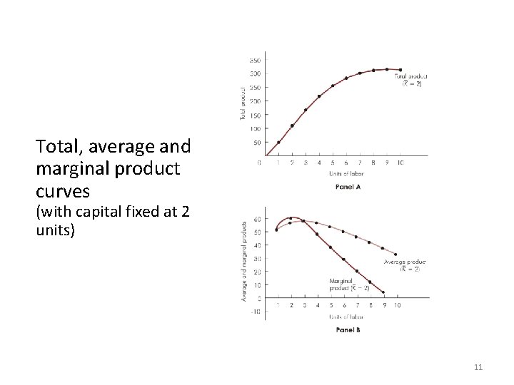
Total, average and marginal product curves (with capital fixed at 2 units) 11

Law of Diminishing Marginal Product • Number of units of the variable input increases, a point will be reached beyond which the marginal product decreases • Other inputs held constant • Increasing, diminishing and negative marginal product situations 12

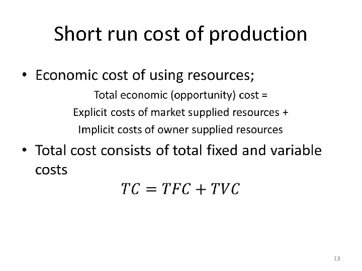
Short run cost of production • 13

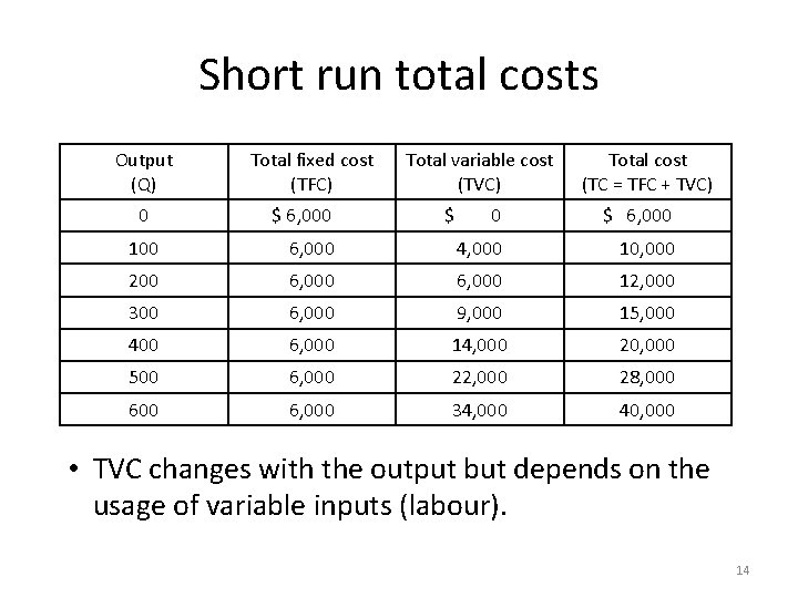
Short run total costs Output (Q) 0 Total fixed cost (TFC) Total variable cost (TVC) Total cost (TC = TFC + TVC) $ 6, 000 $ 0 $ 6, 000 100 6, 000 4, 000 10, 000 200 6, 000 12, 000 300 6, 000 9, 000 15, 000 400 6, 000 14, 000 20, 000 500 6, 000 22, 000 28, 000 6, 000 34, 000 40, 000 • TVC changes with the output but depends on the usage of variable inputs (labour). 14

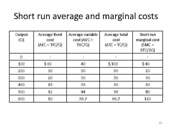
Short run average and marginal costs Output (Q) Average fixed cost (AFC = TFC/Q) Average variable cost (AVC = TVC/Q) Average total cost (ATC = TC/Q) Short run marginal cost (SMC = ∆TC/∆Q) 0 - - 100 $ 60 40 $ 100 $ 40 200 30 30 60 20 30 50 30 400 15 35 50 50 500 12 44 56 80 600 10 56. 7 66. 7 120 15

Short run average and marginal cost curves • SMC curve crosses AVC and ATC curves at their respective minimum points. • So, AVC and ATC falling when SMC is less than those. 16

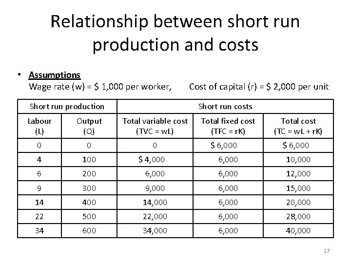
Relationship between short run production and costs • Assumptions Wage rate (w) = $ 1, 000 per worker, Cost of capital (r) = $ 2, 000 per unit Short run production Short run costs Labour (L) Output (Q) Total variable cost (TVC = w. L) 0 0 0 4 100 6 Total fixed cost (TFC = r. K) Total cost (TC = w. L + r. K) $ 6, 000 $ 4, 000 6, 000 10, 000 200 6, 000 12, 000 9 300 9, 000 6, 000 15, 000 14 400 14, 000 6, 000 20, 000 22 500 22, 000 6, 000 28, 000 34 600 34, 000 6, 000 40, 000 17

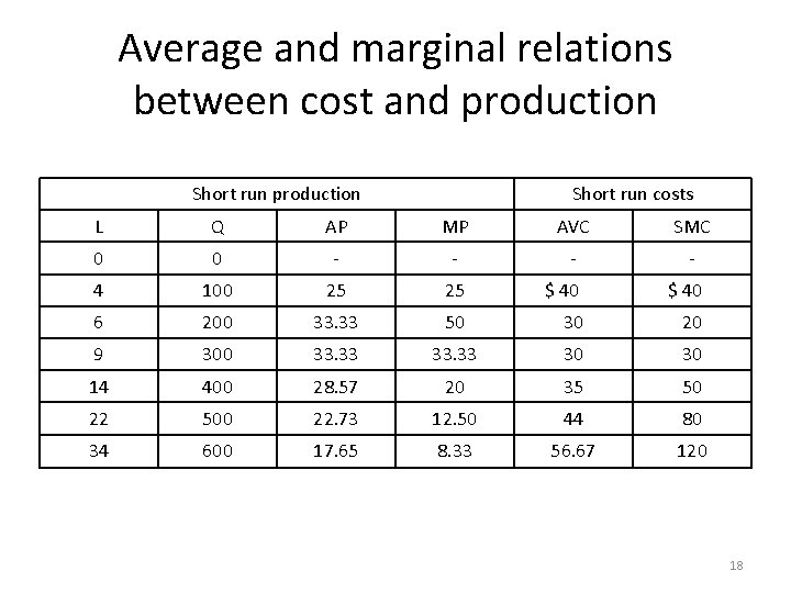
Average and marginal relations between cost and production Short run costs L Q AP MP AVC SMC 0 0 - - 4 100 25 25 $ 40 6 200 33. 33 50 30 20 9 300 33. 33 30 30 14 400 28. 57 20 35 50 22 500 22. 73 12. 50 44 80 34 600 17. 65 8. 33 56. 67 120 18

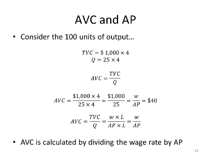
AVC and AP • 19

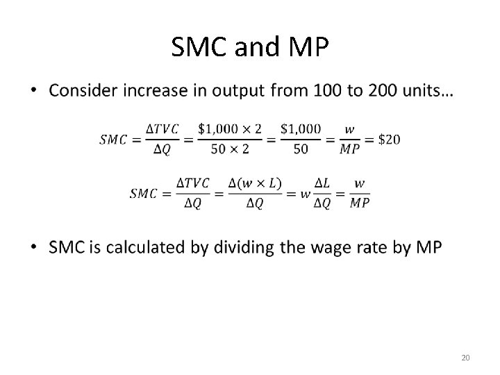
SMC and MP • 20

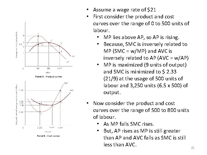
• Assume a wage rate of $21 • First consider the product and cost curves over the range of 0 to 500 units of labour. • MP lies above AP, so AP is rising. • Because, SMC is inversely related to MP (SMC = w/MP) and AVC is inversely related to AP (AVC = w/AP) • MP is maximized (9 units of output) and SMC is minimized to $ 2. 33 (21/9) at the usage of 500 units of labour and 3, 250 units (6. 5 x 500) of output. • Now consider the product and cost curves over the range of 500 to 800 units of labour. • As MP falls SMC rises. • But, AP rises as MP is still greater than AP and AVC falls as SMC is still less than AVC. 21

Implications for managers… • Relations between production and cost curves in the short run involves the effect of the law of diminishing marginal product on the marginal cost of production. • In the above example; – At 800 units of labour and 5, 600 units of output, both SMC and AVC are equal ($3) and AVC reaches its minimum. – Beyond this point AP begins to decrease but never becomes negative. However, MP eventually becomes negative. • So…what’s your decision? 22

Production and cost in the long run • Increase in the scale of operations – Need to increase the amount of capital employed – Variability of all factors of production with the output change • Economies of scale • Economies of scope – Reduce the cost of one good by becoming the producer of other related goods in production • Related diversification • Mergers and acquisitions 23

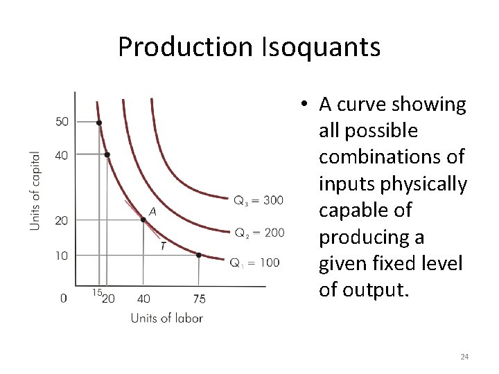
Production Isoquants • A curve showing all possible combinations of inputs physically capable of producing a given fixed level of output. 24

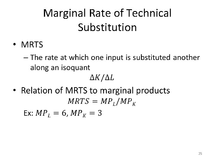
Marginal Rate of Technical Substitution • 25

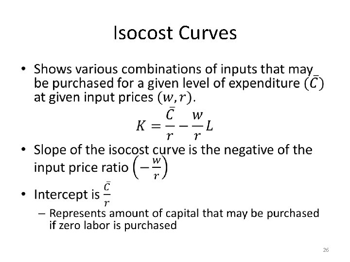
Isocost Curves • 26

Isocost Curves 27

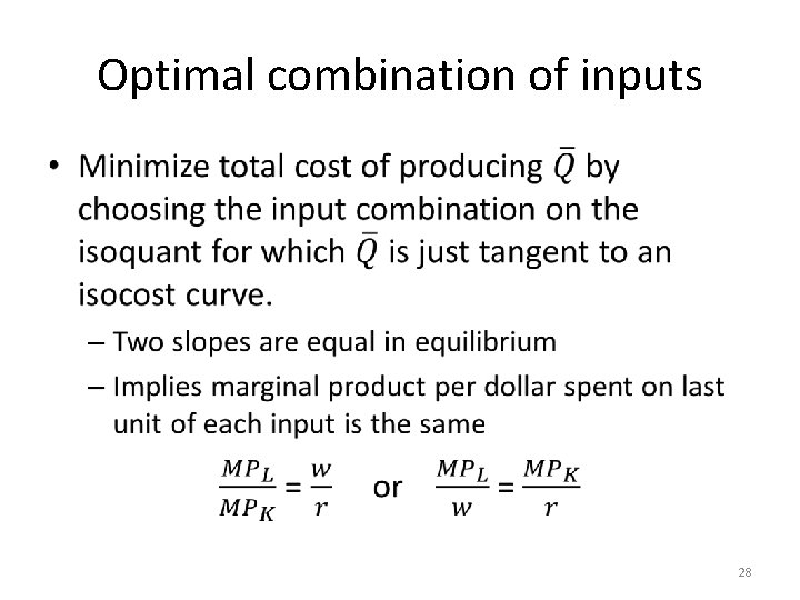
Optimal combination of inputs • 28

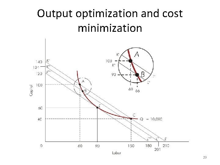
Output optimization and cost minimization 29

Optimization and cost • Expansion path gives the efficient (least-cost) input combinations for every level of output – Derived for a specific set of input prices – Along expansion path, input-price ratio is constant & equal to the MRTS 30

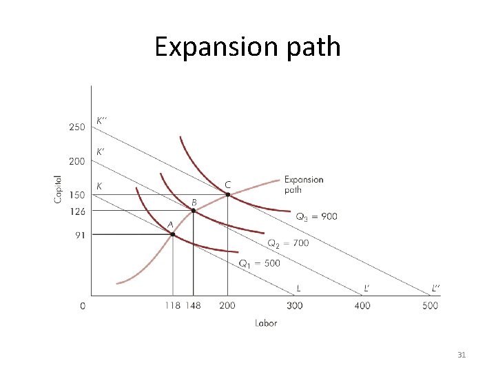
Expansion path 31