Parameter Statistic and Random Samples A parameter is

Parameter, Statistic and Random Samples • A parameter is a number that describes the population. It is a fixed number, but in practice we do not know its value. • A statistic is a function of the sample data, i. e. , it is a quantity whose value can be calculated from the sample data. It is a random variable with a distribution function. Statistics are used to make inference about unknown population parameters. • The random variables X 1, X 2, …, Xn are said to form a (simple) random sample of size n if the Xi’s are independent random variables and each Xi has the sample probability distribution. We say that the Xi’s are iid. STA 286 week 8 1

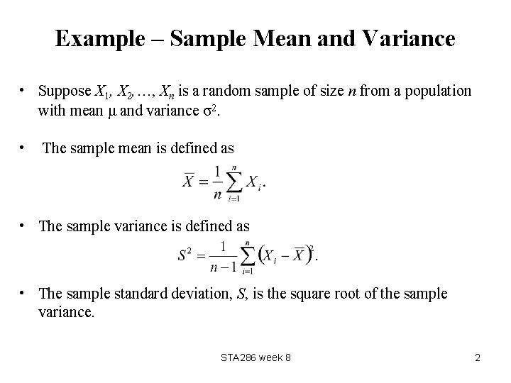
Example – Sample Mean and Variance • Suppose X 1, X 2, …, Xn is a random sample of size n from a population with mean μ and variance σ2. • The sample mean is defined as • The sample variance is defined as • The sample standard deviation, S, is the square root of the sample variance. STA 286 week 8 2

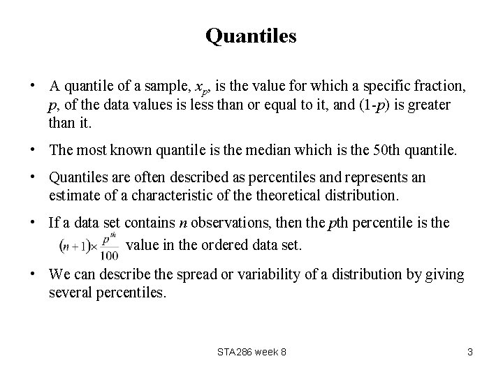
Quantiles • A quantile of a sample, xp, is the value for which a specific fraction, p, of the data values is less than or equal to it, and (1 -p) is greater than it. • The most known quantile is the median which is the 50 th quantile. • Quantiles are often described as percentiles and represents an estimate of a characteristic of theoretical distribution. • If a data set contains n observations, then the pth percentile is the value in the ordered data set. • We can describe the spread or variability of a distribution by giving several percentiles. STA 286 week 8 3

Quartiles • The 25 th percentile is called the first quartile (Q 1). • The 75 th percentile is called the third quartile (Q 3). • Note, the median is the second quartile Q 2. • The distance between the first and third quartiles is called the Interquartile range (IQR) i. e. IQR =Q 3 – Q 1. • The IQR is another measure of spread that is less sensitive to the influence of extreme values. STA 286 week 8 4

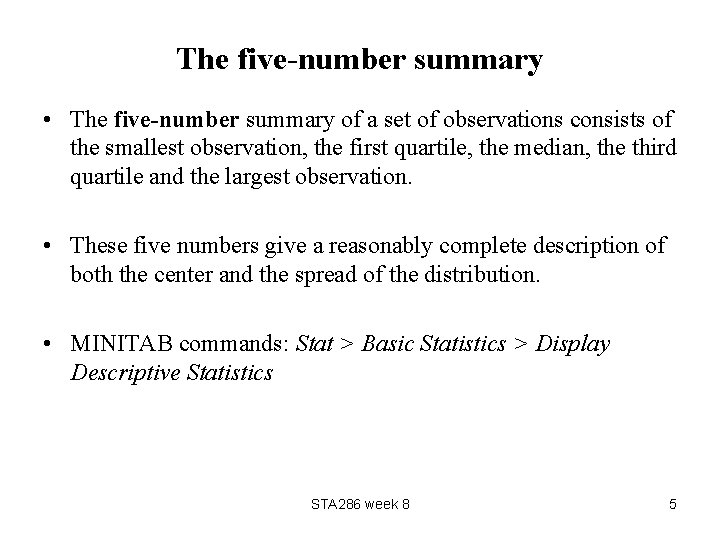
The five-number summary • The five-number summary of a set of observations consists of the smallest observation, the first quartile, the median, the third quartile and the largest observation. • These five numbers give a reasonably complete description of both the center and the spread of the distribution. • MINITAB commands: Stat > Basic Statistics > Display Descriptive Statistics STA 286 week 8 5

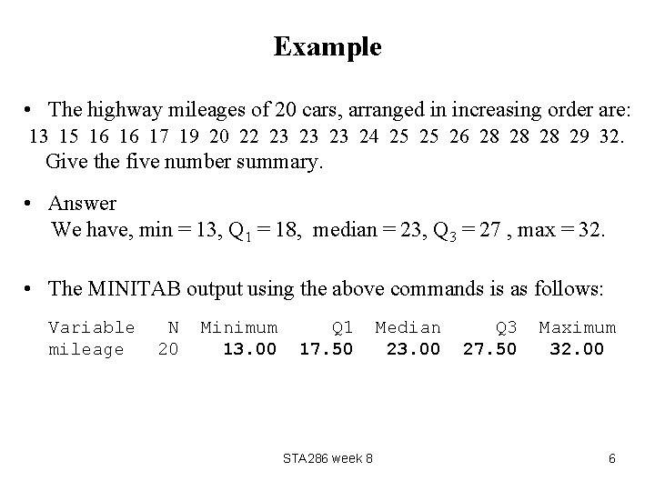
Example • The highway mileages of 20 cars, arranged in increasing order are: 13 15 16 16 17 19 20 22 23 23 23 24 25 25 26 28 28 28 29 32. Give the five number summary. • Answer We have, min = 13, Q 1 = 18, median = 23, Q 3 = 27 , max = 32. • The MINITAB output using the above commands is as follows: Variable mileage N 20 Minimum 13. 00 Q 1 17. 50 STA 286 week 8 Median 23. 00 Q 3 27. 50 Maximum 32. 00 6

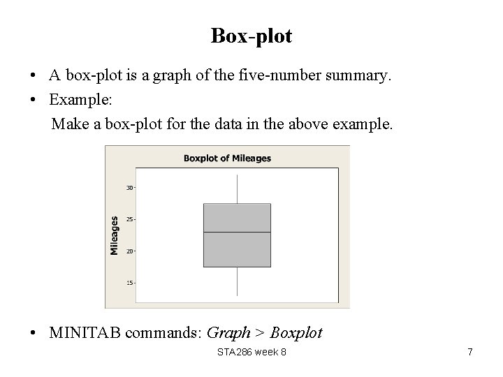
Box-plot • A box-plot is a graph of the five-number summary. • Example: Make a box-plot for the data in the above example. • MINITAB commands: Graph > Boxplot STA 286 week 8 7

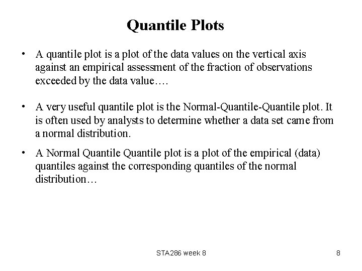
Quantile Plots • A quantile plot is a plot of the data values on the vertical axis against an empirical assessment of the fraction of observations exceeded by the data value…. • A very useful quantile plot is the Normal-Quantile plot. It is often used by analysts to determine whether a data set came from a normal distribution. • A Normal Quantile plot is a plot of the empirical (data) quantiles against the corresponding quantiles of the normal distribution… STA 286 week 8 8

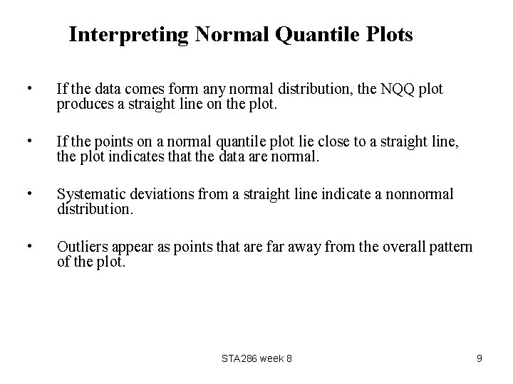
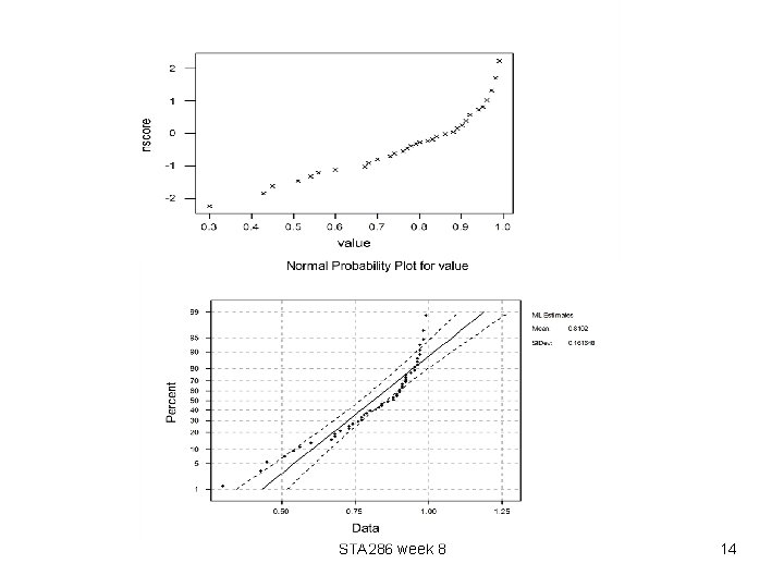
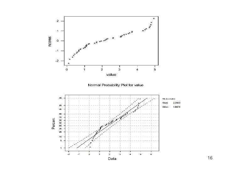
Interpreting Normal Quantile Plots • If the data comes form any normal distribution, the NQQ plot produces a straight line on the plot. • If the points on a normal quantile plot lie close to a straight line, the plot indicates that the data are normal. • Systematic deviations from a straight line indicate a nonnormal distribution. • Outliers appear as points that are far away from the overall pattern of the plot. STA 286 week 8 9

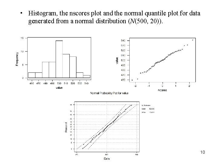
• Histogram, the nscores plot and the normal quantile plot for data generated from a normal distribution (N(500, 20)). STA 286 week 8 10

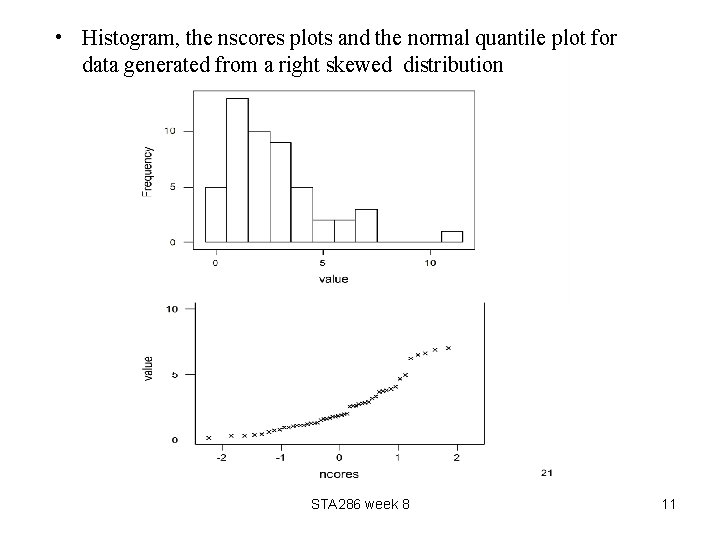
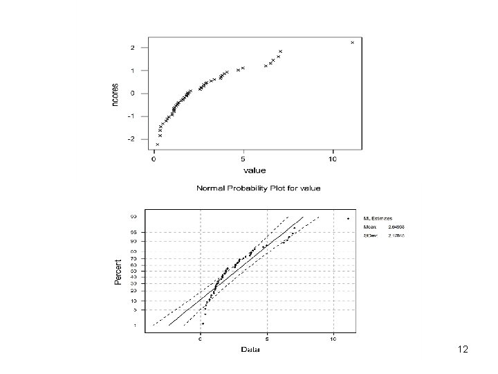
• Histogram, the nscores plots and the normal quantile plot for data generated from a right skewed distribution STA 286 week 8 11

STA 286 week 8 12

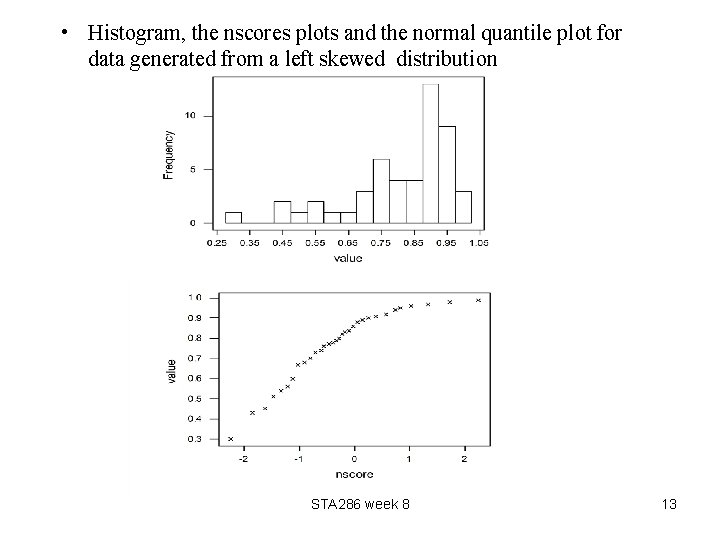
• Histogram, the nscores plots and the normal quantile plot for data generated from a left skewed distribution STA 286 week 8 13

STA 286 week 8 14

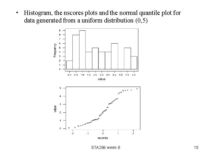
• Histogram, the nscores plots and the normal quantile plot for data generated from a uniform distribution (0, 5) STA 286 week 8 15

STA 286 week 8 16

Sampling Distribution of a Statistic • The sampling distribution of a statistic is the distribution of values taken by the statistic in all possible samples of the same size from the same population. • The distribution function of a statistic is NOT the same as the distribution of the original population that generated the original sample. • The form of theoretical sampling distribution of a statistic will depend upon the distribution of the observable random variables in the sample. STA 286 week 8 17

Sampling from Normal population • Often we assume the random sample X 1, X 2, …Xn is from a normal population with unknown mean μ and variance σ2. • Suppose we are interested in estimating μ and testing whether it is equal to a certain value. For this we need to know the probability distribution of the estimator of μ. STA 286 week 8 18

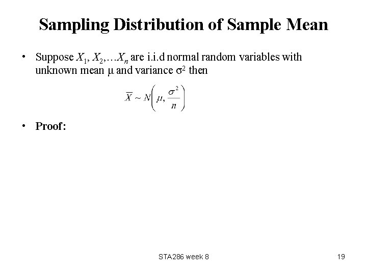
Sampling Distribution of Sample Mean • Suppose X 1, X 2, …Xn are i. i. d normal random variables with unknown mean μ and variance σ2 then • Proof: STA 286 week 8 19

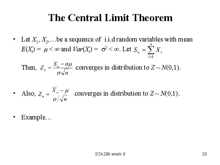
The Central Limit Theorem • Let X 1, X 2, …be a sequence of i. i. d random variables with mean E(Xi) = μ < ∞ and Var(Xi) = σ2 < ∞. Let Then, converges in distribution to Z ~ N(0, 1). • Also, converges in distribution to Z ~ N(0, 1). • Example… STA 286 week 8 20

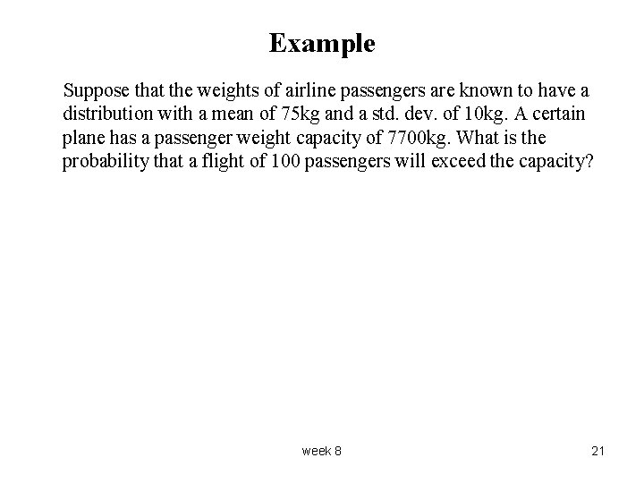
Example Suppose that the weights of airline passengers are known to have a distribution with a mean of 75 kg and a std. dev. of 10 kg. A certain plane has a passenger weight capacity of 7700 kg. What is the probability that a flight of 100 passengers will exceed the capacity? week 8 21

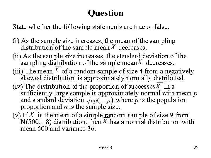
Question State whether the following statements are true or false. (i) As the sample size increases, the mean of the sampling distribution of the sample mean decreases. (ii) As the sample size increases, the standard deviation of the sampling distribution of the sample mean decreases. (iii) The mean of a random sample of size 4 from a negatively skewed distribution is approximately normally distributed. (iv) The distribution of the proportion of successes in a sufficiently large sample is approximately normal with mean p and standard deviation where p is the population proportion and n is the sample size. (v) If is the mean of a simple random sample of size 9 from N(500, 18) distribution, then has a normal distribution with mean 500 and variance 36. week 8 22

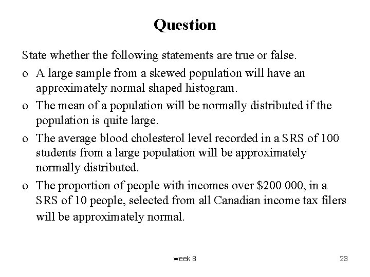
Question State whether the following statements are true or false. o A large sample from a skewed population will have an approximately normal shaped histogram. o The mean of a population will be normally distributed if the population is quite large. o The average blood cholesterol level recorded in a SRS of 100 students from a large population will be approximately normally distributed. o The proportion of people with incomes over $200 000, in a SRS of 10 people, selected from all Canadian income tax filers will be approximately normal. week 8 23

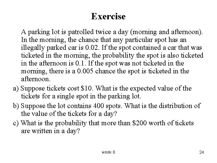
Exercise A parking lot is patrolled twice a day (morning and afternoon). In the morning, the chance that any particular spot has an illegally parked car is 0. 02. If the spot contained a car that was ticketed in the morning, the probability the spot is also ticketed in the afternoon is 0. 1. If the spot was not ticketed in the morning, there is a 0. 005 chance the spot is ticketed in the afternoon. a) Suppose tickets cost $10. What is the expected value of the tickets for a single spot in the parking lot. b) Suppose the lot contains 400 spots. What is the distribution of the value of the tickets for a day? c) What is the probability that more than $200 worth of tickets are written in a day? week 8 24

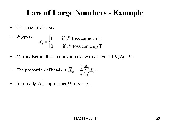
Law of Large Numbers - Example • Toss a coin n times. • Suppose • Xi’s are Bernoulli random variables with p = ½ and E(Xi) = ½. • The proportion of heads is • Intuitively . approaches ½ as n ∞. STA 286 week 8 25

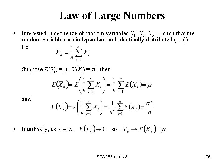
Law of Large Numbers • Interested in sequence of random variables X 1, X 2, X 3, … such that the random variables are independent and identically distributed (i. i. d). Let Suppose E(Xi) = μ , V(Xi) = σ2, then and • Intuitively, as n ∞, so STA 286 week 8 26

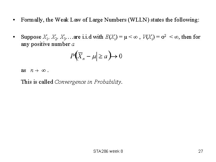
• Formally, the Weak Law of Large Numbers (WLLN) states the following: • Suppose X 1, X 2, X 3, …are i. i. d with E(Xi) = μ < ∞ , V(Xi) = σ2 < ∞, then for any positive number a as n ∞. This is called Convergence in Probability. STA 286 week 8 27

Recall - The Chi Square distribution • If Z ~ N(0, 1) then, X = Z 2 has a Chi-Square distribution with parameter 1, i. e. , • Can proof this using change of variable theorem for univariate random variables. • The moment generating function of X is • If , all independent then • Proof… STA 286 week 8 28

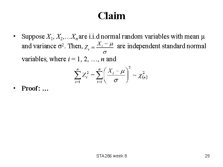
Claim • Suppose X 1, X 2, …Xn are i. i. d normal random variables with mean μ and variance σ2. Then, are independent standard normal variables, where i = 1, 2, …, n and • Proof: … STA 286 week 8 29

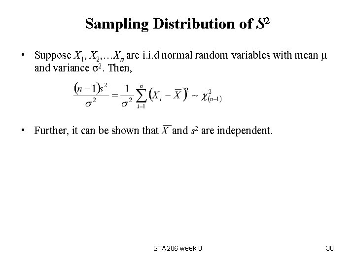
Sampling Distribution of S 2 • Suppose X 1, X 2, …Xn are i. i. d normal random variables with mean μ and variance σ2. Then, • Further, it can be shown that and s 2 are independent. STA 286 week 8 30

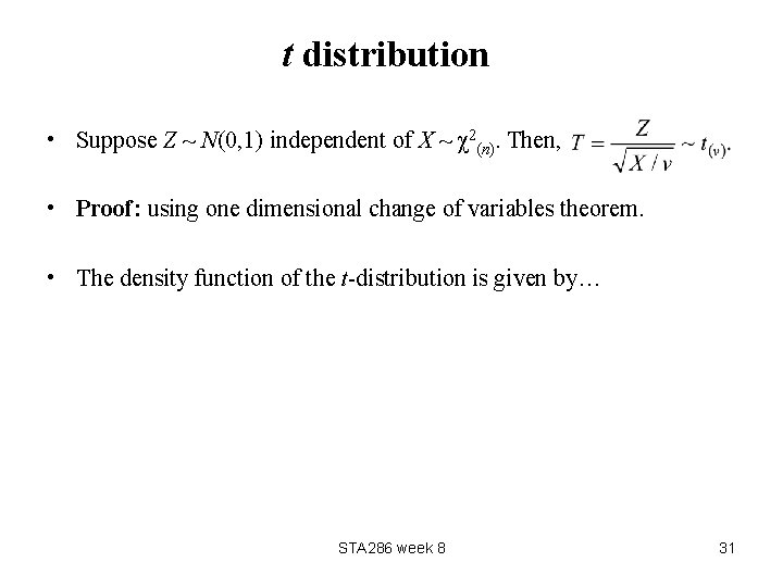
t distribution • Suppose Z ~ N(0, 1) independent of X ~ χ2(n). Then, • Proof: using one dimensional change of variables theorem. • The density function of the t-distribution is given by… STA 286 week 8 31

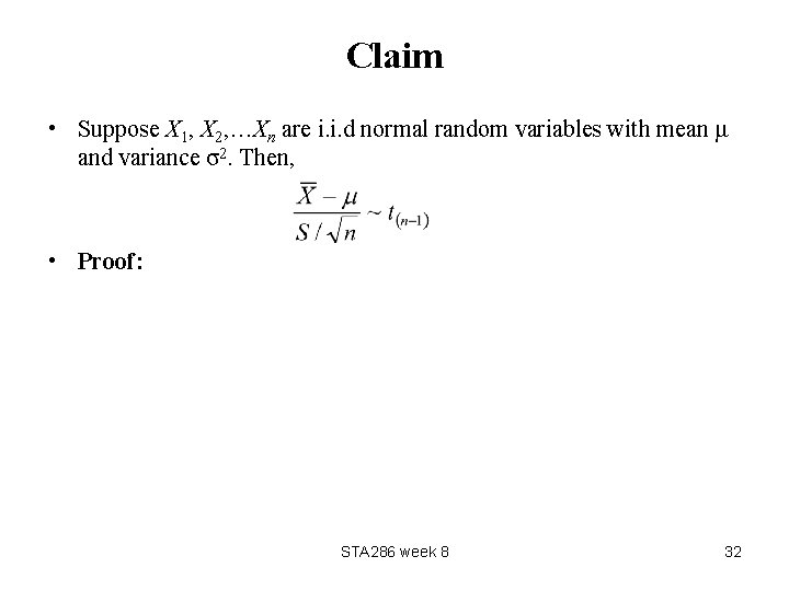
Claim • Suppose X 1, X 2, …Xn are i. i. d normal random variables with mean μ and variance σ2. Then, • Proof: STA 286 week 8 32

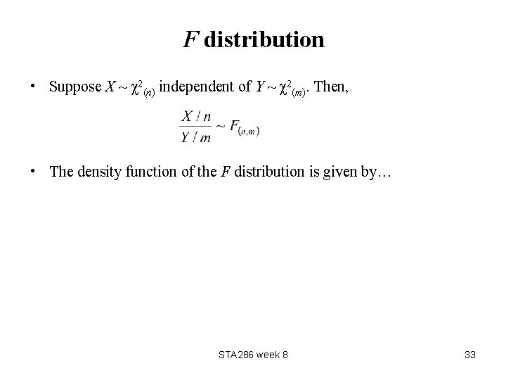
F distribution • Suppose X ~ χ2(n) independent of Y ~ χ2(m). Then, • The density function of the F distribution is given by… STA 286 week 8 33

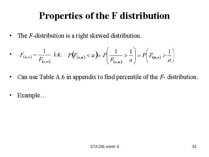
Properties of the F distribution • The F-distribution is a right skewed distribution. • i. e. • Can use Table A. 6 in appendix to find percentile of the F- distribution. • Example… STA 286 week 8 34