Logics for Data and Knowledge Representation Application of

Logics for Data and Knowledge Representation Application of (Ground) Class. L

Outline q Ontologies q Lightweight Ontologies q Classifications q Optimization q Document of Classifications Classification in LOs q Query-answering q Semantic 2 in LOs Matching

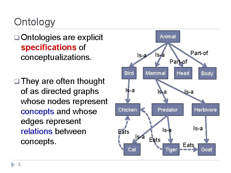
Ontology q Ontologies are explicit specifications of conceptualizations. are often thought of as directed graphs whose nodes represent concepts and whose edges represent relations between concepts. Animal Is-a Part-of Bird Mammal Is-a Head Body q They Chicken Eats Is-a Cat 3 Predator Eats Tiger Is-a Herbivore Is-a Eats Goat

Concept q The notion of concept is understood as defined in Knowledge Representation, i. e. , as a set of objects or individuals. q This set is called the concept extension or the concept interpretation. q Concepts are often lexically defined, i. e. they have natural language names which are used to describe the concept extensions. 4

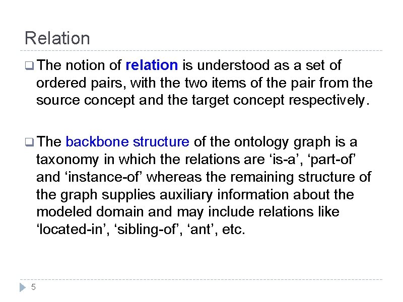
Relation q The notion of relation is understood as a set of ordered pairs, with the two items of the pair from the source concept and the target concept respectively. q The backbone structure of the ontology graph is a taxonomy in which the relations are ‘is-a’, ‘part-of’ and ‘instance-of’ whereas the remaining structure of the graph supplies auxiliary information about the modeled domain and may include relations like ‘located-in’, ‘sibling-of’, ‘ant’, etc. 5

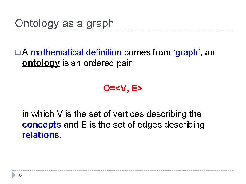
Ontology as a graph q. A mathematical definition comes from ‘graph’, an ontology is an ordered pair O=<V, E> in which V is the set of vertices describing the concepts and E is the set of edges describing relations. 6

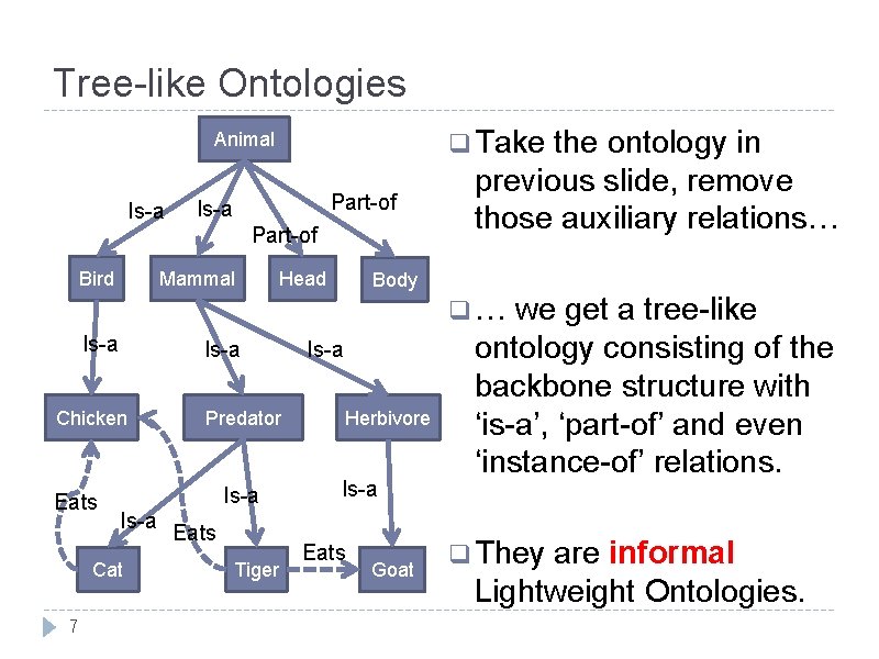
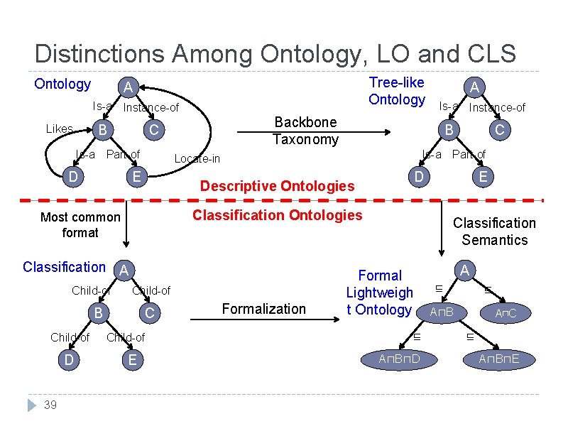
Tree-like Ontologies q Take Animal Is-a Part-of Bird Mammal Head the ontology in previous slide, remove those auxiliary relations… Body q… Is-a Chicken Eats Is-a Cat 7 Predator Eats Tiger Is-a Herbivore Is-a Eats Goat we get a tree-like ontology consisting of the backbone structure with ‘is-a’, ‘part-of’ and even ‘instance-of’ relations. q They are informal Lightweight Ontologies.

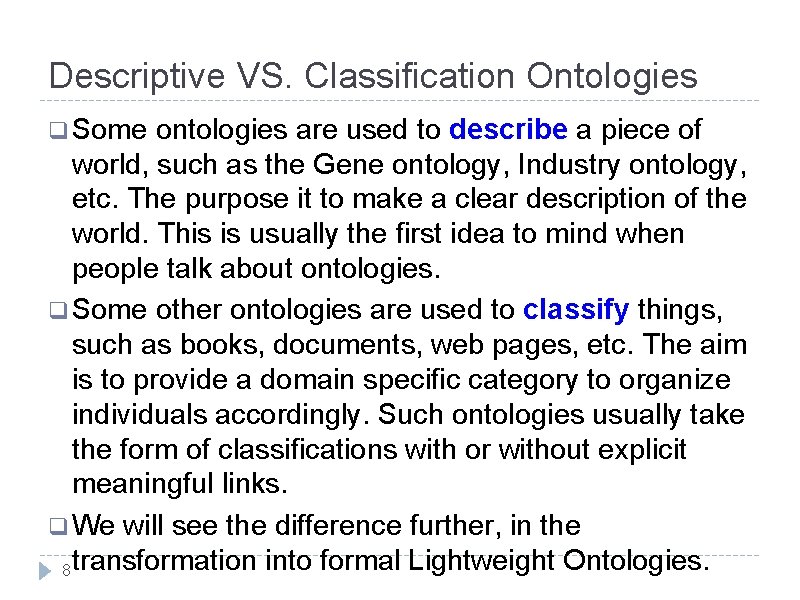
Descriptive VS. Classification Ontologies q Some ontologies are used to describe a piece of world, such as the Gene ontology, Industry ontology, etc. The purpose it to make a clear description of the world. This is usually the first idea to mind when people talk about ontologies. q Some other ontologies are used to classify things, such as books, documents, web pages, etc. The aim is to provide a domain specific category to organize individuals accordingly. Such ontologies usually take the form of classifications with or without explicit meaningful links. q We will see the difference further, in the 8 transformation into formal Lightweight Ontologies.

Why ‘Lightweight’ Ontologies? Two observations: 1. Majority of existing ontologies are ‘simple’ taxonomies or classifications, i. e. , categories to classify resources. 2. Ontologies with arbitrary relations do exist, but no intuitively reasoning techniques support such ontologies in general. … so we need ‘lightweight’ ontologies. 9

Outline q Ontologies q Lightweight Ontologies q Classifications q Optimization q Document of Classifications Classification in LOs q Query-answering q Semantic 10 in LOs Matching

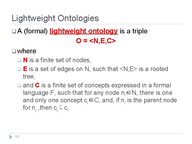
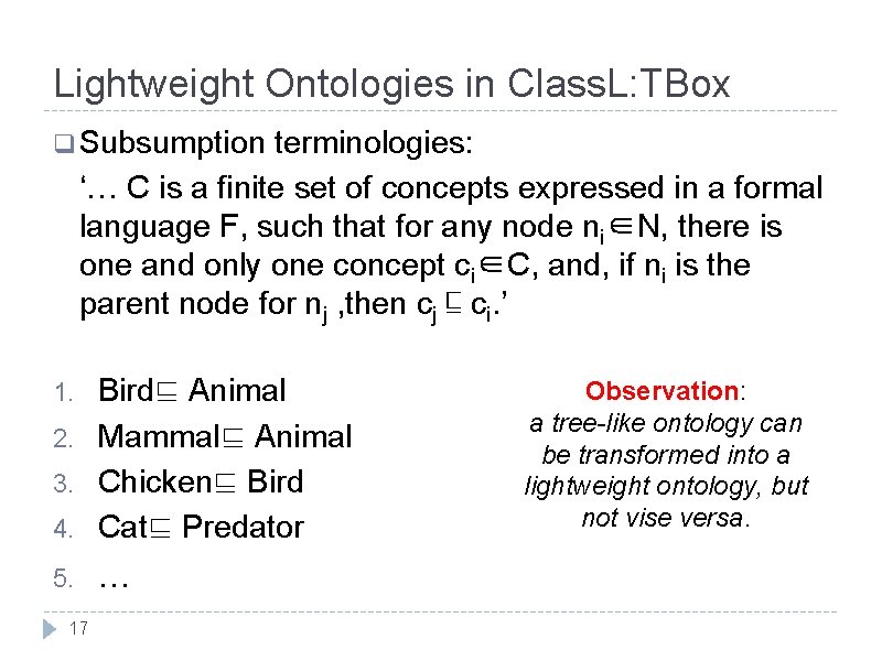
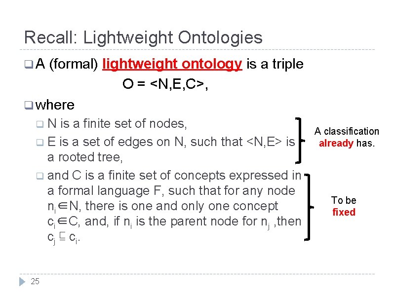
Lightweight Ontologies q. A (formal) lightweight ontology is a triple O = <N, E, C> q where q. N is a finite set of nodes, q E is a set of edges on N, such that <N, E> is a rooted tree, q and C is a finite set of concepts expressed in a formal language F, such that for any node ni∈N, there is one and only one concept ci∈C, and, if ni is the parent node for nj , then cj ⊑ ci. 11

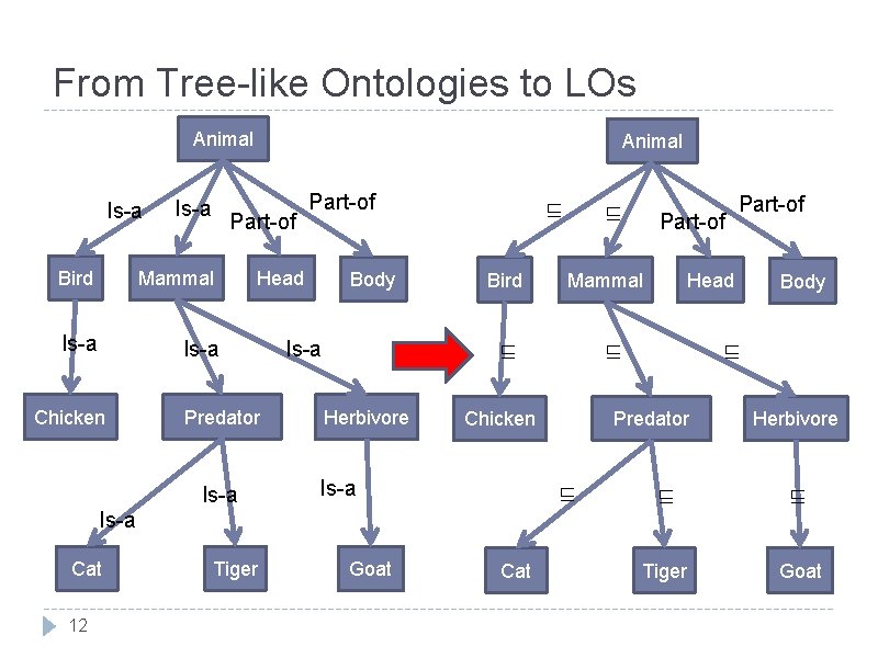
From Tree-like Ontologies to LOs Animal Is-a Part-of Bird Mammal Is-a Chicken Animal Part-of Head Predator Is-a Body ⊑ Bird Herbivore 12 Tiger Goat Cat Body ⊑ Predator ⊑ Part-of Head ⊑ Chicken Is-a Part-of Mammal ⊑ Is-a Cat ⊑ Herbivore ⊑ ⊑ Tiger Goat

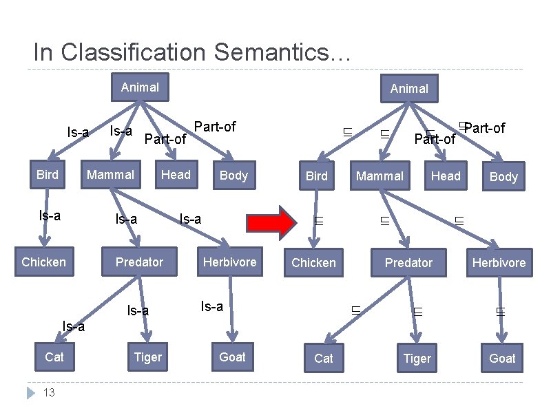
In Classification Semantics… Animal Is-a Part-of Bird Mammal Is-a Chicken Animal Part-of Head Predator Is-a Body ⊑ Bird Herbivore Is-a 13 Tiger Goat Body ⊑ Predator ⊑ Cat Head ⊑ Chicken Is-a Cat Mammal ⊑ Is-a ⊑Part-of ⊑ Herbivore ⊑ ⊑ Tiger Goat

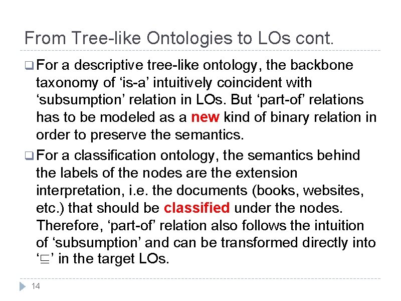
From Tree-like Ontologies to LOs cont. q For a descriptive tree-like ontology, the backbone taxonomy of ‘is-a’ intuitively coincident with ‘subsumption’ relation in LOs. But ‘part-of’ relations has to be modeled as a new kind of binary relation in order to preserve the semantics. q For a classification ontology, the semantics behind the labels of the nodes are the extension interpretation, i. e. the documents (books, websites, etc. ) that should be classified under the nodes. Therefore, ‘part-of’ relation also follows the intuition of ‘subsumption’ and can be transformed directly into ‘⊑’ in the target LOs. 14

Populated (Lightweight) Ontologies q In Information Retrieval, the term classification is seen as the process of arranging a set of objects (e. g. , documents) into categories or classes. q. A classification Ontology is said populated if a set of objects have been classified under ‘proper’ nodes. q Thus a populated (Lightweight) Ontology consists a new type of links: instance-of. 15

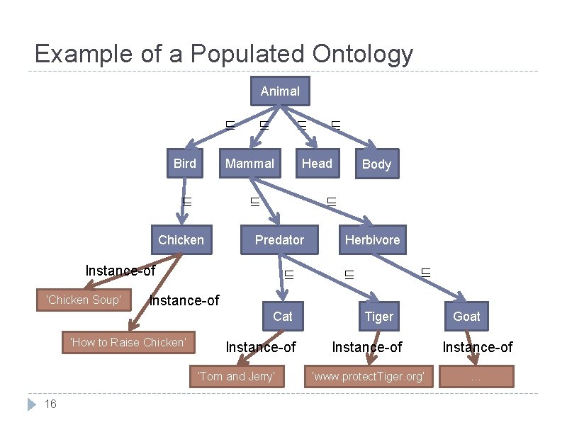
Example of a Populated Ontology Animal ⊑ Bird ⊑ ⊑ Mammal ⊑ Predator ⊑ Herbivore ⊑ ⊑ Instance-of Cat ‘How to Raise Chicken’ Instance-of ‘Tom and Jerry’ 16 Body ⊑ Instance-of ‘Chicken Soup’ Head ⊑ Chicken ⊑ Tiger Goat Instance-of ‘www. protect. Tiger. org’ …

Lightweight Ontologies in Class. L: TBox q Subsumption terminologies: ‘… C is a finite set of concepts expressed in a formal language F, such that for any node ni∈N, there is one and only one concept ci∈C, and, if ni is the parent node for nj , then cj ⊑ ci. ’ 4. Bird⊑ Animal Mammal⊑ Animal Chicken⊑ Bird Cat⊑ Predator 5. … 1. 2. 3. 17 Observation: a tree-like ontology can be transformed into a lightweight ontology, but not vise versa.

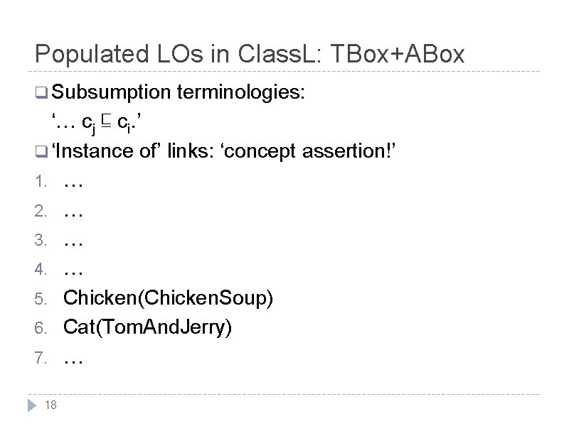
Populated LOs in Class. L: TBox+ABox q Subsumption terminologies: ‘… cj ⊑ ci. ’ q ‘Instance of’ links: ‘concept assertion!’ 1. … 2. … 3. … 4. … 5. Chicken(Chicken. Soup) 6. Cat(Tom. And. Jerry) 7. … 18

Outline q Ontologies q Lightweight Ontologies q Classifications q Optimization q Document of Classifications Classification in LOs q Query-answering q Semantic 19 in LOs Matching

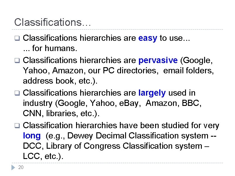
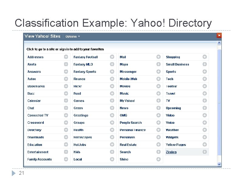
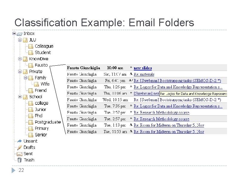
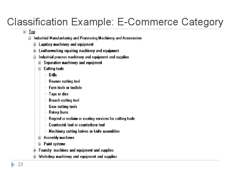
Classifications… q q Classifications hierarchies are easy to use. . . for humans. Classifications hierarchies are pervasive (Google, Yahoo, Amazon, our PC directories, email folders, address book, etc. ). Classifications hierarchies are largely used in industry (Google, Yahoo, e. Bay, Amazon, BBC, CNN, libraries, etc. ). Classification hierarchies have been studied for very long (e. g. , Dewey Decimal Classification system -DCC, Library of Congress Classification system – LCC, etc. ). 20

Classification Example: Yahoo! Directory 21

Classification Example: Email Folders 22

Classification Example: E-Commerce Category 23

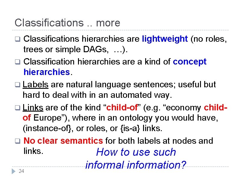
Classifications. . more Classifications hierarchies are lightweight (no roles, trees or simple DAGs, …). q Classification hierarchies are a kind of concept hierarchies. q Labels are natural language sentences; useful but hard to deal with in an automated way. q Links are of the kind “child-of” (e. g. “economy childof Europe”), where in an ontology you would have, (instance-of}, or roles, or {is-a} links. q No clear semantics for both labels at nodes and links. How to use such q 24 informal information?

Recall: Lightweight Ontologies q. A (formal) lightweight ontology is a triple O = <N, E, C>, q where q. N is a finite set of nodes, q E is a set of edges on N, such that <N, E> is a rooted tree, q and C is a finite set of concepts expressed in a formal language F, such that for any node ni∈N, there is one and only one concept ci∈C, and, if ni is the parent node for nj , then cj ⊑ ci. 25 A classification already has. To be fixed

What do LOs Bring? q We know that a lightweight ontology is a formal conceptualization of a domain in terms of concepts and {is-a, instance-of} relationships. q Lightweight ontologies (LOs) add a formal semantics and {instance-of} relationships to classification hierarchies. q In 26 short: LOs make classifications formal!

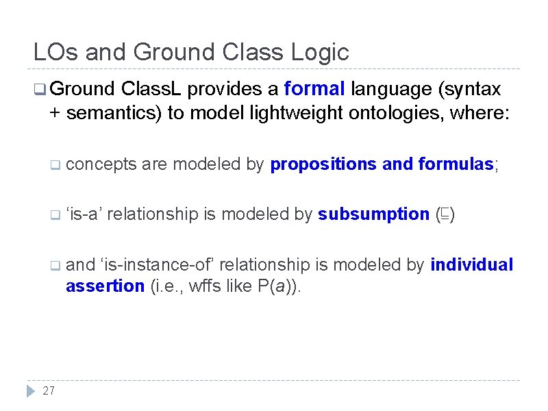
LOs and Ground Class Logic q Ground Class. L provides a formal language (syntax + semantics) to model lightweight ontologies, where: q concepts q ‘is-a’ q and are modeled by propositions and formulas; relationship is modeled by subsumption (⊑) ‘is-instance-of’ relationship is modeled by individual assertion (i. e. , wffs like P(a)). 27

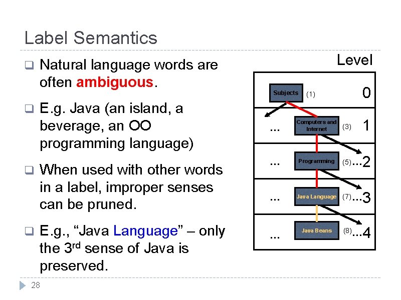
Label Semantics q q Natural language words are often ambiguous. E. g. Java (an island, a beverage, an OO programming language) When used with other words in a label, improper senses can be pruned. E. g. , “Java Language” – only the 3 rd sense of Java is preserved. 28 Level Subjects 0 (1) 1 … Computers and Internet … Programming (5) … … Java Language (7) … Java Beans (8)… … (3) 2 3 4

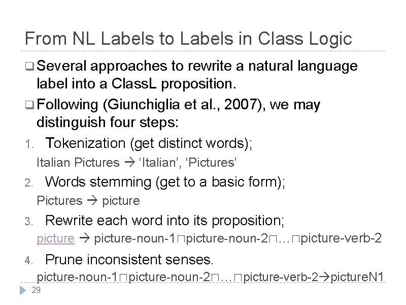
From NL Labels to Labels in Class Logic q Several approaches to rewrite a natural language label into a Class. L proposition. q Following (Giunchiglia et al. , 2007), we may distinguish four steps: 1. Tokenization (get distinct words); Italian Pictures ‘Italian’, ‘Pictures’ Words stemming (get to a basic form); 2. Pictures picture Rewrite each word into its proposition; 3. picture-noun-1⊓picture-noun-2⊓…⊓picture-verb-2 Prune inconsistent senses. 4. picture-noun-1⊓picture-noun-2⊓…⊓picture-verb-2 picture. N 1 29

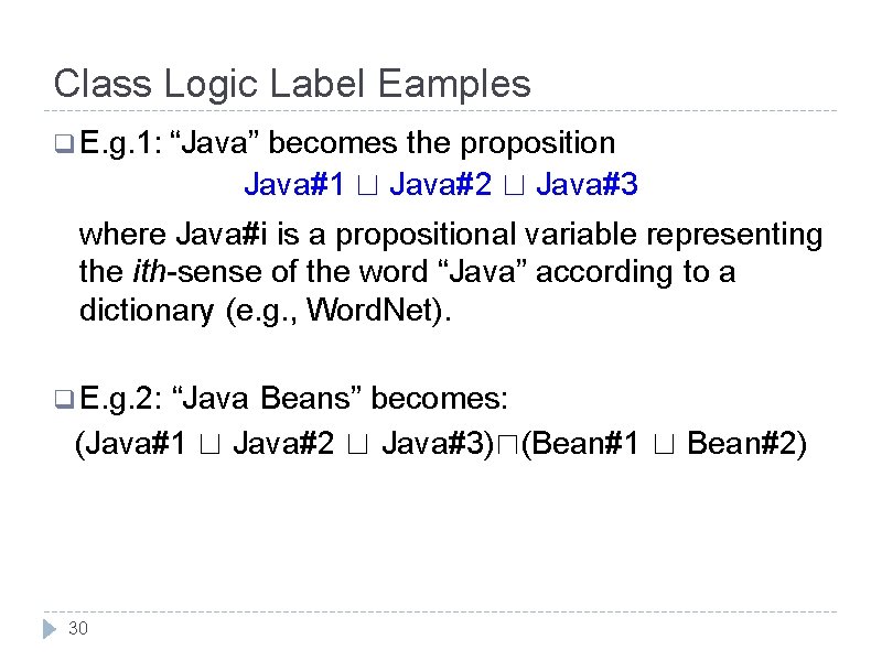
Class Logic Label Eamples q E. g. 1: “Java” becomes the proposition Java#1 ⊔ Java#2 ⊔ Java#3 where Java#i is a propositional variable representing the ith-sense of the word “Java” according to a dictionary (e. g. , Word. Net). q E. g. 2: “Java Beans” becomes: (Java#1 ⊔ Java#2 ⊔ Java#3)⊓(Bean#1 ⊔ Bean#2) 30

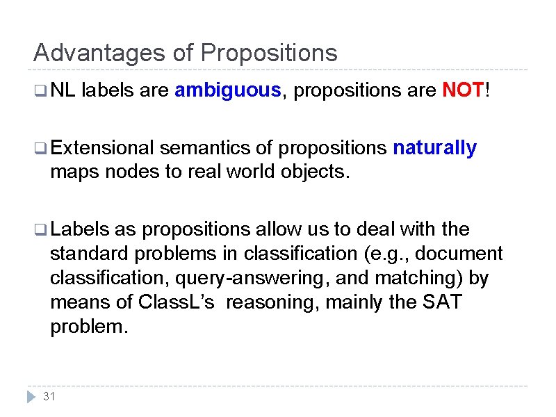
Advantages of Propositions q NL labels are ambiguous, propositions are NOT! q Extensional semantics of propositions naturally maps nodes to real world objects. q Labels as propositions allow us to deal with the standard problems in classification (e. g. , document classification, query-answering, and matching) by means of Class. L’s reasoning, mainly the SAT problem. 31

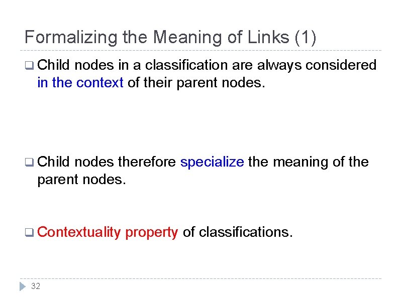
Formalizing the Meaning of Links (1) q Child nodes in a classification are always considered in the context of their parent nodes. q Child nodes therefore specialize the meaning of the parent nodes. q Contextuality 32 property of classifications.

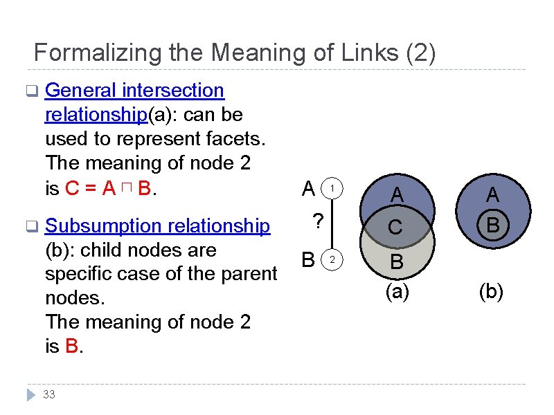
Formalizing the Meaning of Links (2) q q General intersection relationship(a): can be used to represent facets. The meaning of node 2 is C = A ⊓ B. Subsumption relationship (b): child nodes are specific case of the parent nodes. The meaning of node 2 is B. 33 A 1 ? B 2 A C A B B (a) (b)

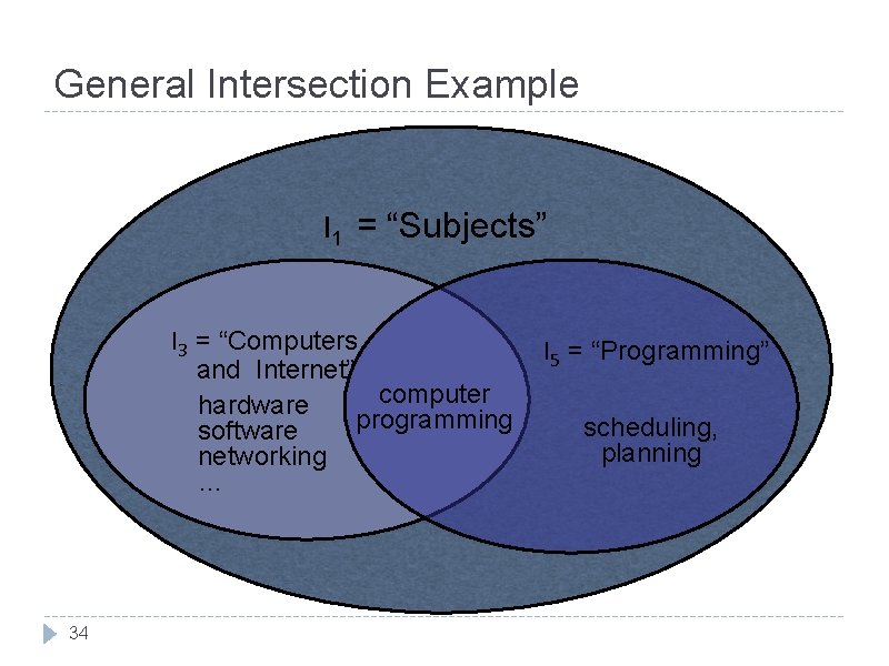
General Intersection Example l 1 = “Subjects” l 3 = “Computers and Internet” computer hardware programming software networking … 34 l 5 = “Programming” scheduling, planning

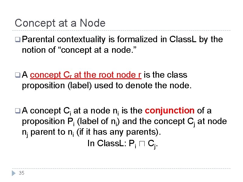
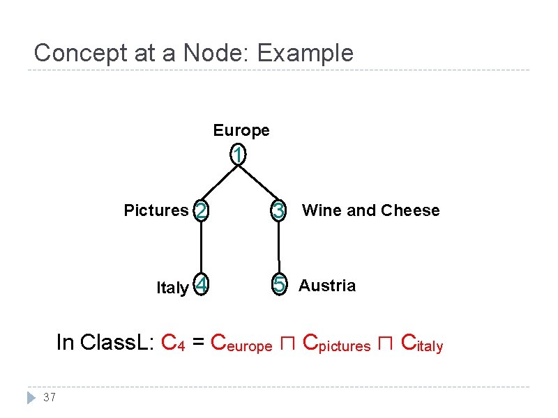
Concept at a Node q Parental contextuality is formalized in Class. L by the notion of “concept at a node. ” q. A concept Cr at the root node r is the class proposition (label) used to denote the node. q. A concept Ci at a node ni is the conjunction of a proposition Pi (label of ni) and the concept Cj at node nj parent to ni (if it has any parents). In Class. L: Pi ⊓ Cj. 35

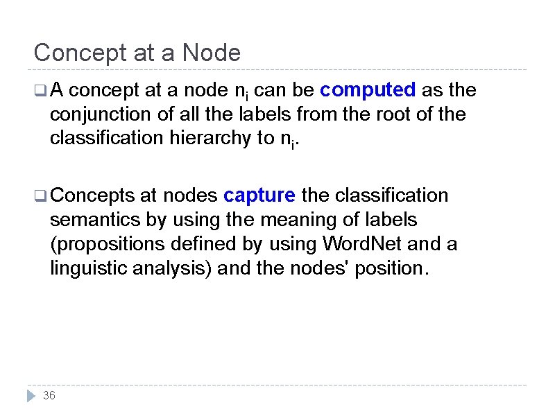
Concept at a Node q. A concept at a node ni can be computed as the conjunction of all the labels from the root of the classification hierarchy to ni. q Concepts at nodes capture the classification semantics by using the meaning of labels (propositions defined by using Word. Net and a linguistic analysis) and the nodes' position. 36

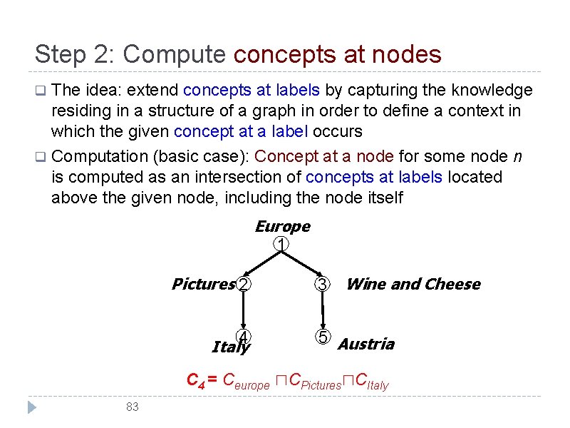
Concept at a Node: Example Europe 1 Pictures 2 3 Wine and Cheese Italy 4 5 Austria In Class. L: C 4 = Ceurope ⊓ Cpictures ⊓ Citaly 37

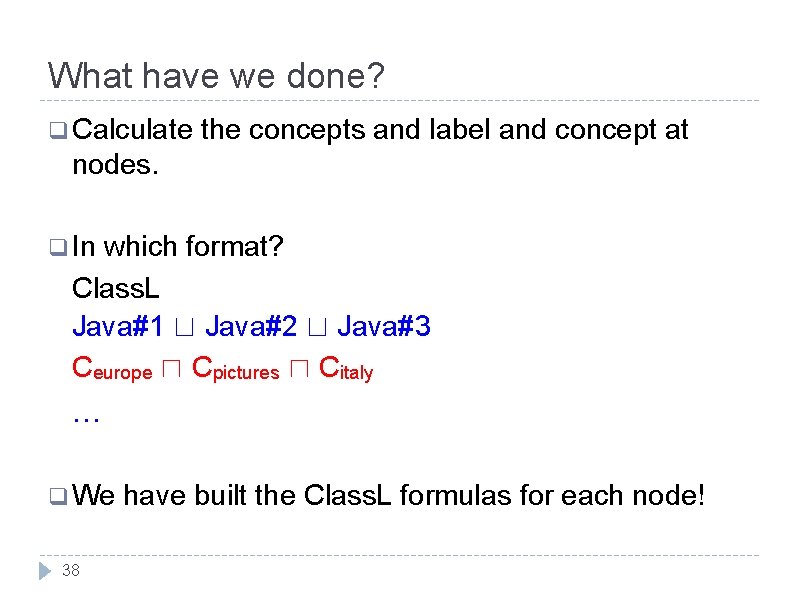
What have we done? q Calculate the concepts and label and concept at nodes. q In which format? Class. L Java#1 ⊔ Java#2 ⊔ Java#3 Ceurope ⊓ Cpictures ⊓ Citaly … q We 38 have built the Class. L formulas for each node!

Distinctions Among Ontology, LO and CLS Ontology Tree-like Ontology A Is-a Instance-of B Likes D Classification A Child-of D 39 D E Classification Ontologies Child-of B C Child-of E C Is-a Part-of Descriptive Ontologies Most common format Child-of B Locate-in E Is-a Instance-of Backbone Taxonomy C Is-a Part-of A Formalization Classification Semantics Formal Lightweigh t Ontology ⊑ A⊓B⊓D A ⊑ ⊑ A⊓B A⊓C ⊑ A⊓B⊓E

Outline q Ontologies q Lightweight Ontologies q Classifications q Optimization q Document of Classifications Classification in LOs q Query-answering q Semantic 40 in LOs Matching

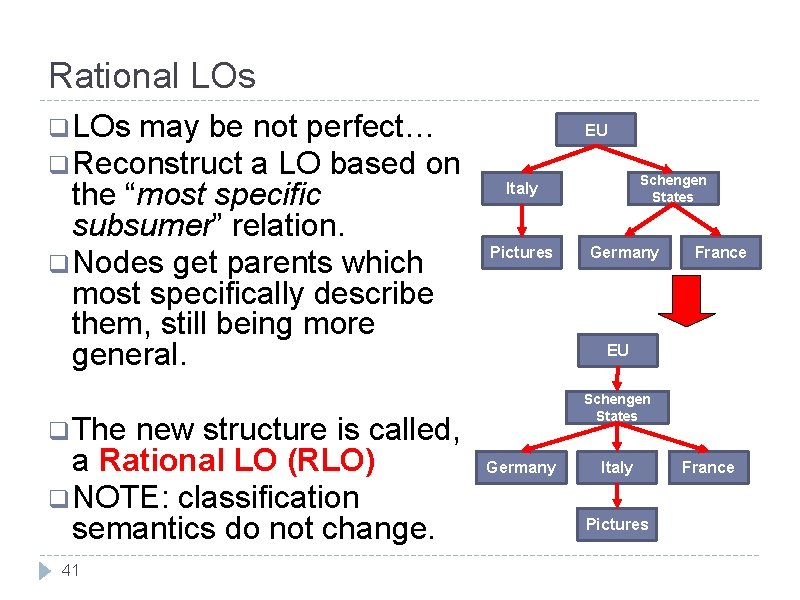
Rational LOs q LOs may be not perfect… q Reconstruct a LO based on the “most specific subsumer” relation. q Nodes get parents which most specifically describe them, still being more general. new structure is called, a Rational LO (RLO) q NOTE: classification semantics do not change. EU Pictures Germany France EU Schengen States q The 41 Schengen States Italy Germany Italy Pictures France

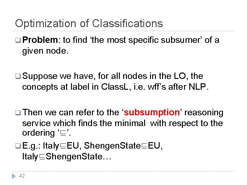
Optimization of Classifications q Problem: to find ‘the most specific subsumer’ of a given node. q Suppose we have, for all nodes in the LO, the concepts at label in Class. L, i. e. wff’s after NLP. q Then we can refer to the ‘subsumption’ reasoning service which finds the minimal with respect to the ordering ‘⊑’. q E. g. : Italy⊑EU, Shengen. State⊑EU, Italy⊑Shengen. State… 42

Outline q Ontologies q Lightweight Ontologies q Classifications q Optimization q Document of Classifications Classification in LOs q Query-answering q Semantic 43 in LOs Matching

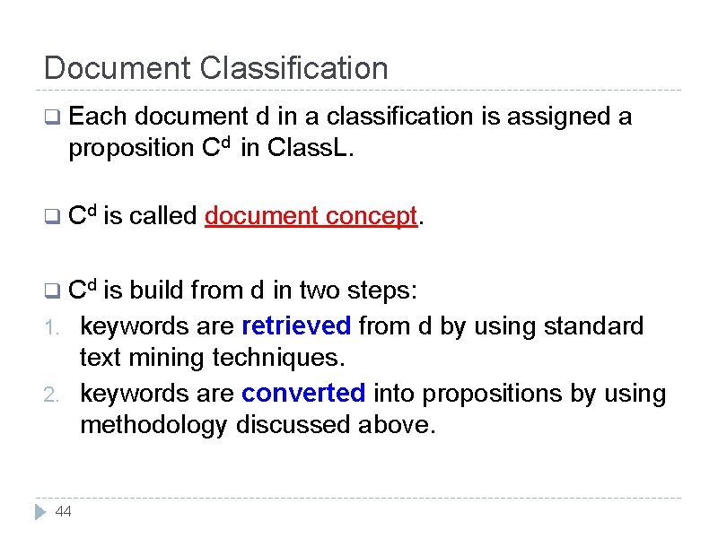
Document Classification q Each document d in a classification is assigned a proposition Cd in Class. L. q Cd is called document concept. q Cd is build from d in two steps: keywords are retrieved from d by using standard text mining techniques. keywords are converted into propositions by using methodology discussed above. 1. 2. 44

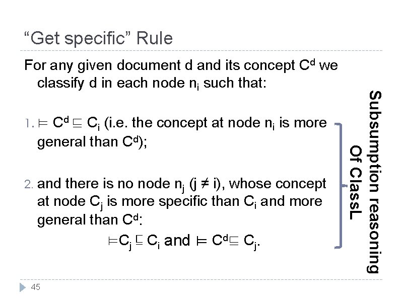
“Get specific” Rule 1. ⊨ Cd ⊑ Ci (i. e. the concept at node ni is more general than Cd); 2. and there is no node nj (j ≠ i), whose concept at node Cj is more specific than Ci and more general than Cd: ⊨Cj ⊑ Ci and ⊨ Cd⊑ Cj. 45 Subsumption reasoning Of Class. L For any given document d and its concept Cd we classify d in each node ni such that:

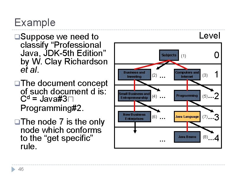
Example we need to classify “Professional Java, JDK-5 th Edition” by W. Clay Richardson et al. Level q Suppose document concept of such document d is: Cd = Java#3⊓ Programming#2. Subjects node 7 is the only node which conforms to the “get specific” rule. 46 1 Business and Investing (2) … Computers and Internet Small Business and Entrepreneurship (4) … Programming (5) … New Business Enterprises (6) … Java Language (7) … Java Beans (8)… q The 0 (1) … (3) 2 3 4

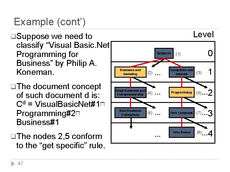
Example (cont’) we need to classify “Visual Basic. Net Programming for Business” by Philip A. Koneman. Level q Suppose q The document concept of such document d is: Cd = Visual. Basic. Net#1⊓ Programming#2⊓ Business#1 q The nodes 2, 5 conform to the “get specific” rule. 47 Subjects 0 (1) 1 Business and Investing (2) … Computers and Internet Small Business and Entrepreneurship (4) … Programming (5) … New Business Enterprises (6) … Java Language (7) … Java Beans (8)… … (3) 2 3 4

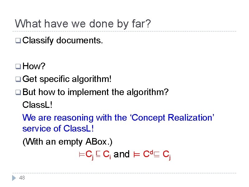
What have we done by far? q Classify documents. q How? q Get specific algorithm! q But how to implement the algorithm? Class. L! We are reasoning with the ‘Concept Realization’ service of Class. L! (With an empty ABox. ) ⊨Cj ⊑ Ci and ⊨ Cd⊑ Cj 48

Outline q Ontologies q Lightweight Ontologies q Classifications q Optimization q Document of Classifications Classification in LOs q Query-answering q Semantic 49 in LOs Matching

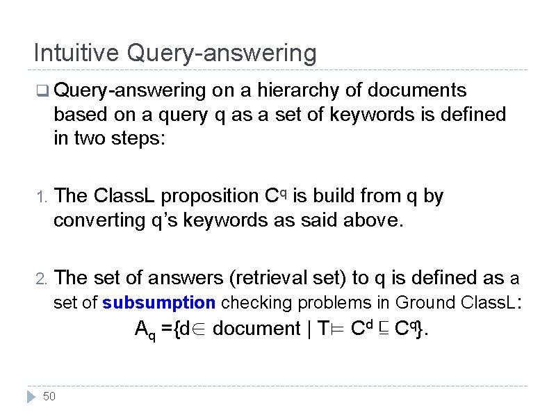
Intuitive Query-answering q Query-answering on a hierarchy of documents based on a query q as a set of keywords is defined in two steps: 1. The Class. L proposition Cq is build from q by converting q’s keywords as said above. 2. The set of answers (retrieval set) to q is defined as a set of subsumption checking problems in Ground Class. L: Aq ={d∈ document | T⊨ Cd ⊑ Cq}. 50

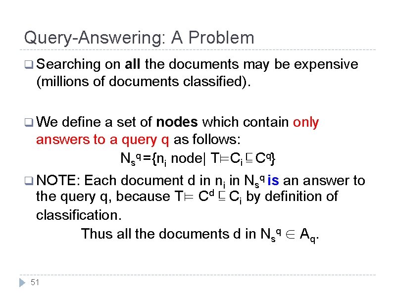
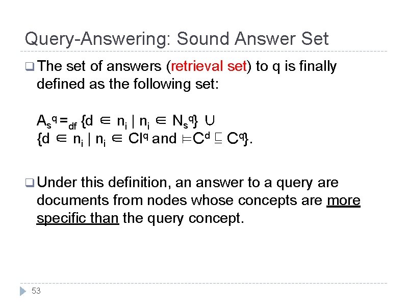
Query-Answering: A Problem q Searching on all the documents may be expensive (millions of documents classified). q We define a set of nodes which contain only answers to a query q as follows: Nsq ={ni node| T⊨Ci ⊑ Cq} q NOTE: Each document d in ni in Nsq is an answer to the query q, because T⊨ Cd ⊑ Ci by definition of classification. Thus all the documents d in Nsq ∈ Aq. 51

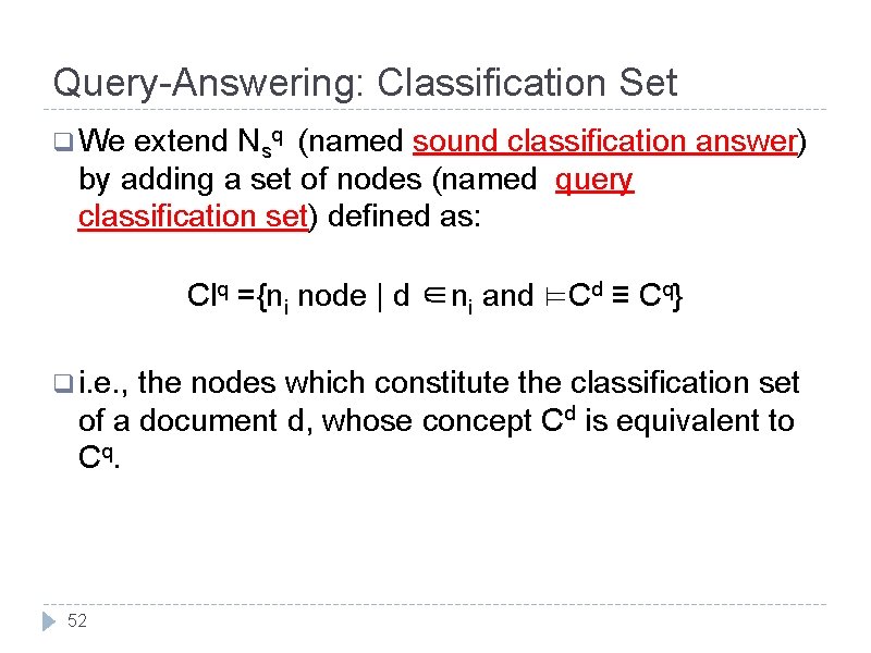
Query-Answering: Classification Set q We extend Nsq (named sound classification answer) by adding a set of nodes (named query classification set) defined as: Clq ={ni node | d ∈ni and ⊨Cd ≡ Cq} q i. e. , the nodes which constitute the classification set of a document d, whose concept Cd is equivalent to C q. 52

Query-Answering: Sound Answer Set q The set of answers (retrieval set) to q is finally defined as the following set: Asq =df {d ∈ ni | ni ∈ Nsq} ∪ {d ∈ ni | ni ∈ Clq and ⊨Cd ⊑ Cq}. q Under this definition, an answer to a query are documents from nodes whose concepts are more specific than the query concept. 53

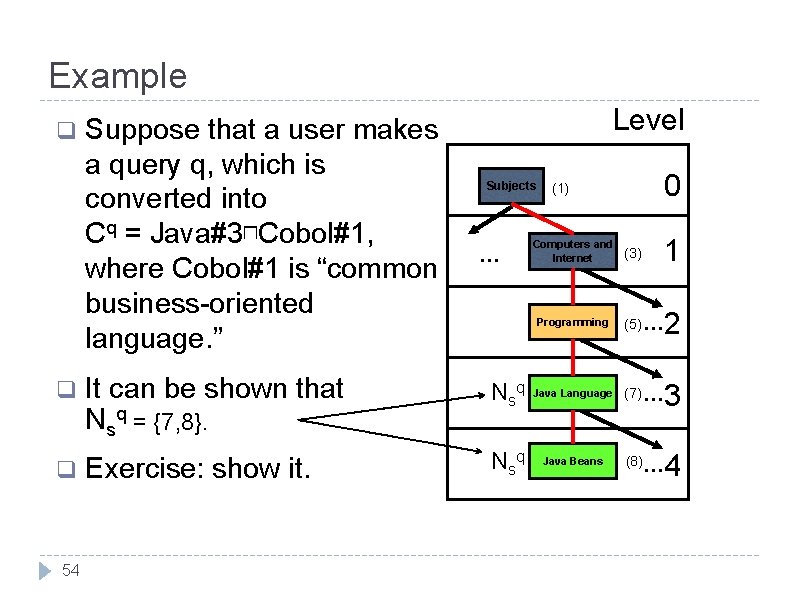
Example q q q 54 Suppose that a user makes a query q, which is converted into Cq = Java#3⊓Cobol#1, where Cobol#1 is “common business-oriented language. ” Level Subjects … 0 (1) Computers and Internet (3) 1 2 Programming (5) … It can be shown that Nsq = {7, 8}. N sq Java Language (7) … Exercise: show it. N sq Java Beans (8)… 3 4

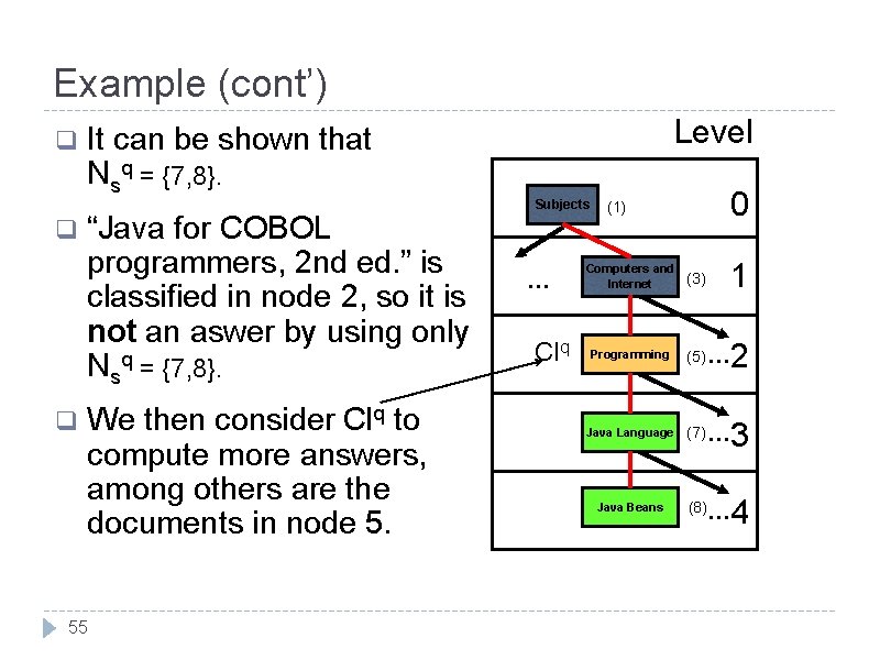
Example (cont’) q q q Level It can be shown that Nsq = {7, 8}. “Java for COBOL programmers, 2 nd ed. ” is classified in node 2, so it is not an aswer by using only Nsq = {7, 8}. We then consider Clq to compute more answers, among others are the documents in node 5. 55 Subjects … Clq 0 (1) Computers and Internet (3) 1 2 Programming (5) … Java Language (7) … Java Beans (8)… 3 4

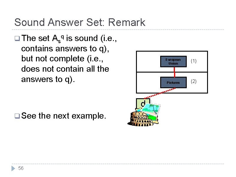
Sound Answer Set: Remark q The set Asq is sound (i. e. , contains answers to q), but not complete (i. e. , does not contain all the answers to q). d q See 56 the next example. European Union (1) Pictures (2)

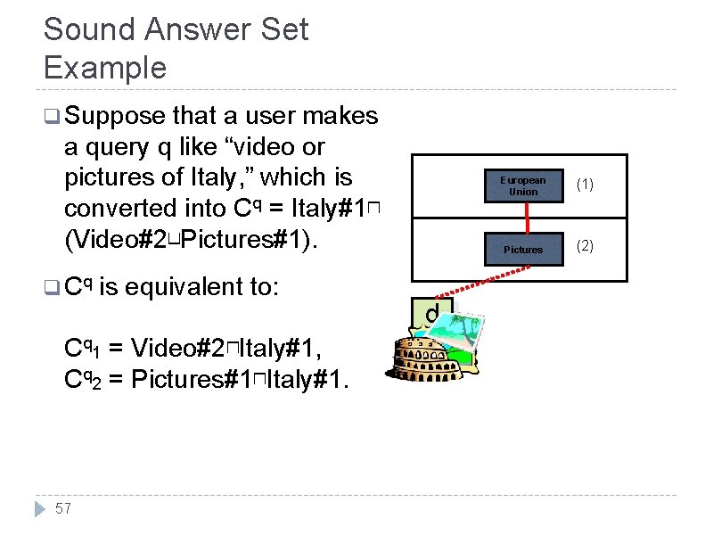
Sound Answer Set Example q Suppose that a user makes a query q like “video or pictures of Italy, ” which is converted into Cq = Italy#1⊓ (Video#2⊔Pictures#1). q Cq is equivalent to: Cq 1 = Video#2⊓Italy#1, Cq 2 = Pictures#1⊓Italy#1. 57 d European Union (1) Pictures (2)

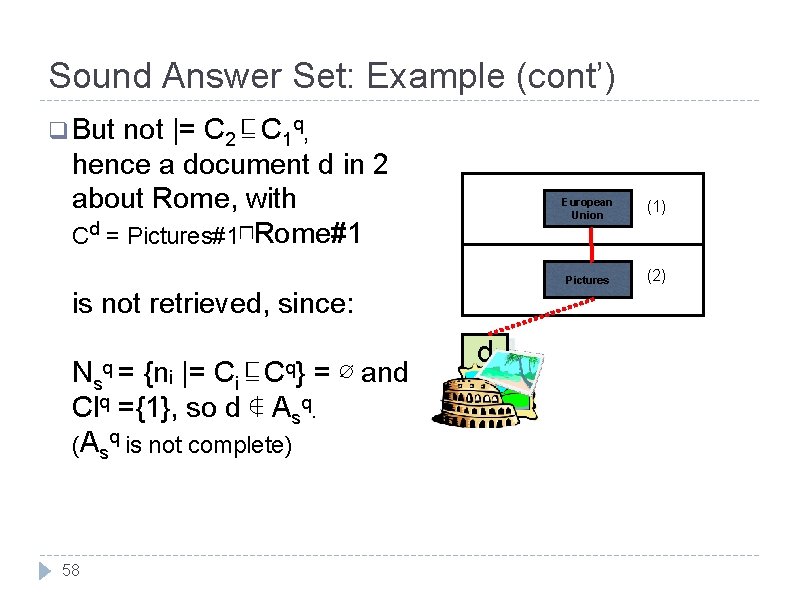
Sound Answer Set: Example (cont’) q But not |= C 2 ⊑ C 1 q, hence a document d in 2 about Rome, with Cd = Pictures#1⊓Rome#1 is not retrieved, since: Nsq = {ni |= Ci ⊑ Cq} = Clq ={1}, so d ∉ Asq. (Asq is not complete) 58 ∅ and d European Union (1) Pictures (2)

Some Comments q The edge structure of a LO is not considered for document classification, neither for query answering. q The edges information becomes redundant, as it is implicitly encoded in the “concept at a node” notion. q There are more than one way to build a LO from a set of concepts at nodes. 59

What have we done in Query Answering? q Find the set of documents. q How? q Find q But the concept that is subsumed by the query. how to implement it? Class. L! We are reasoning with the ‘Concept subsumption’ service of Class. L! ⊨Cd ⊑ Cq 60

Outline q Ontologies q Lightweight Ontologies q Classifications q Optimization q Document of Classifications Classification in LOs q Query-answering q Semantic 61 in LOs Matching

Date: a matching? 62

Why Matching? q Most popular knowledge can be represented as graphs. The heterogeneity between knowledge graphs demands the exposition of relations, such as semantically equivalent. q Some popular situations that can be modeled as a matching problem are: Concept matching in semantic networks. Schema matching in distributed databases. Ontology matching (ontology “alignment”) in the Semantic Web. 63

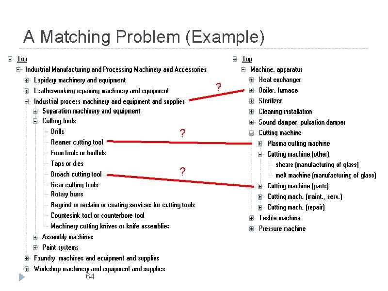
A Matching Problem (Example) ? ? ? 64

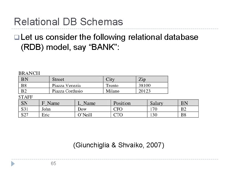
Relational DB Schemas q Let us consider the following relational database (RDB) model, say “BANK”: (Giunchiglia & Shvaiko, 2007) 65

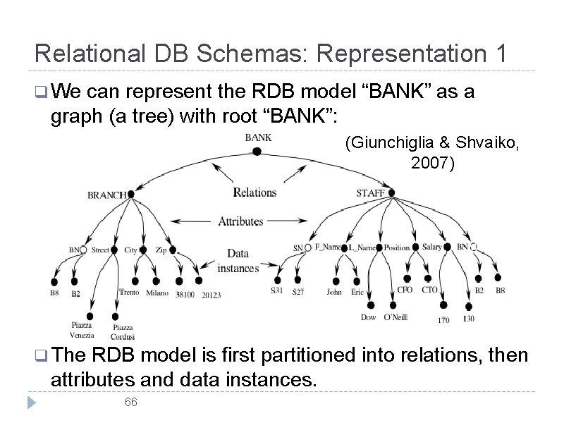
Relational DB Schemas: Representation 1 q We can represent the RDB model “BANK” as a graph (a tree) with root “BANK”: (Giunchiglia & Shvaiko, 2007) q The RDB model is first partitioned into relations, then attributes and data instances. 66

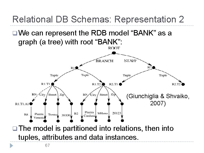
Relational DB Schemas: Representation 2 q We can represent the RDB model “BANK” as a graph (a tree) with root “BANK”: (Giunchiglia & Shvaiko, 2007) q The model is partitioned into relations, then into tuples, attributes and data instances. 67

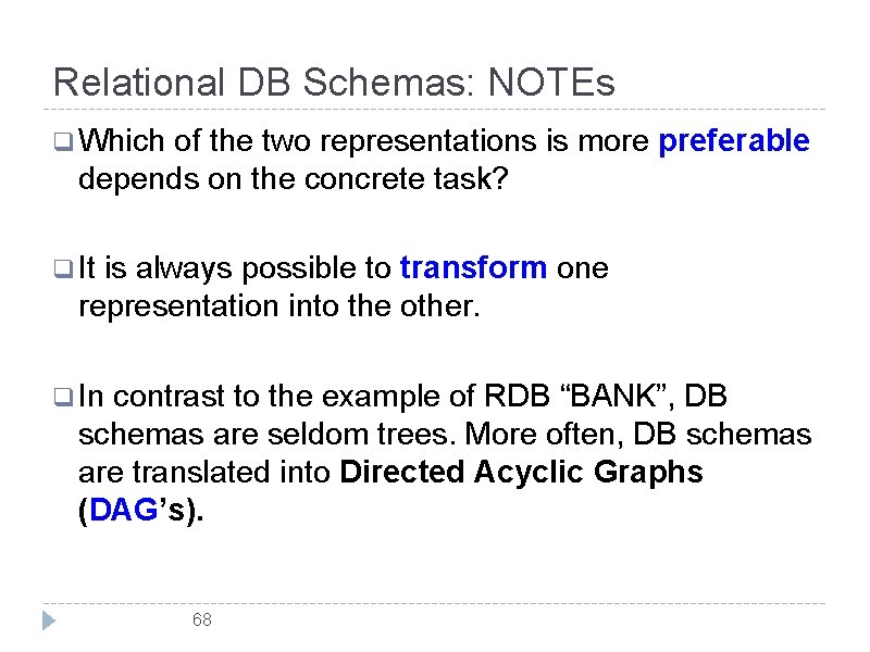
Relational DB Schemas: NOTEs q Which of the two representations is more preferable depends on the concrete task? q It is always possible to transform one representation into the other. q In contrast to the example of RDB “BANK”, DB schemas are seldom trees. More often, DB schemas are translated into Directed Acyclic Graphs (DAG’s). 68

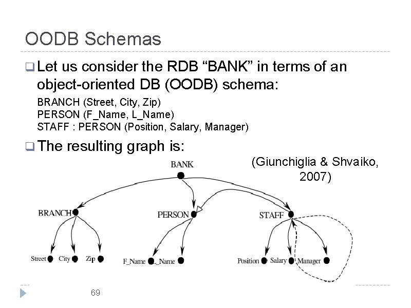
OODB Schemas q Let us consider the RDB “BANK” in terms of an object-oriented DB (OODB) schema: BRANCH (Street, City, Zip) PERSON (F_Name, L_Name) STAFF : PERSON (Position, Salary, Manager) q The resulting graph is: (Giunchiglia & Shvaiko, 2007) 69

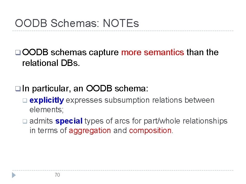
OODB Schemas: NOTEs q OODB schemas capture more semantics than the relational DBs. q In particular, an OODB schema: q explicitly expresses subsumption relations between elements; q admits special types of arcs for part/whole relationships in terms of aggregation and composition. 70

Semi-structured Data q Neither RDBs nor OODBs capture all the features of semi-structured or unstructured data (Buneman, 1997): q semi-structured data do not possess a regular structure (schemaless); q the “structure” of semi-structured data could be partial or even implicit. q Typical examples are: HTML and XML. 71

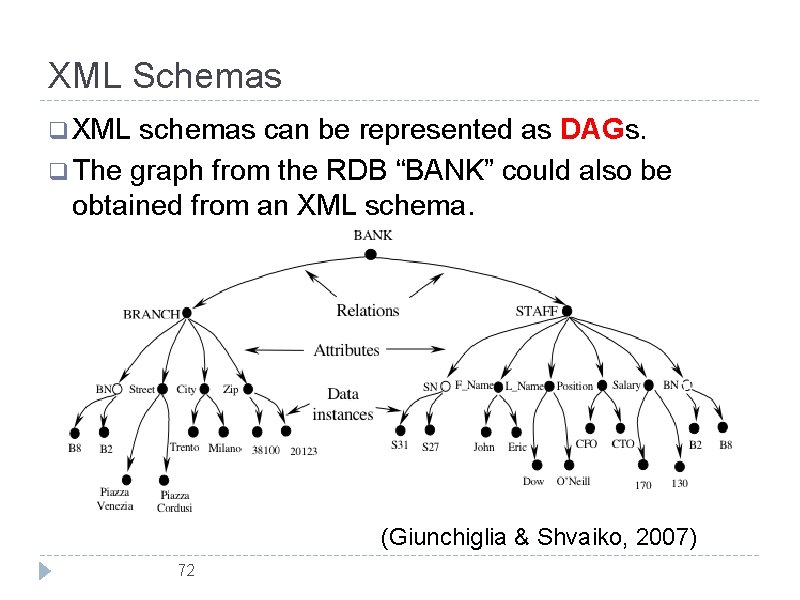
XML Schemas q XML schemas can be represented as DAGs. q The graph from the RDB “BANK” could also be obtained from an XML schema. (Giunchiglia & Shvaiko, 2007) 72

XML Schemas: NOTEs q Often XML schemas represent hierarchical data models. q In this case the only relationships between the elements are {is-a}. q Attributes in XML are used to represent extra information about data. There are no strict rules telling us when data should be represented as elements, or as attributes. 73

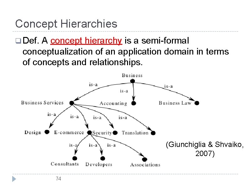
Concept Hierarchies q Def. A concept hierarchy is a semi-formal conceptualization of an application domain in terms of concepts and relationships. (Giunchiglia & Shvaiko, 2007) 74

Concept Hierarchies: NOTEs q Examples are classification hierarchies, e. g. , and directories (catalogs). q Classification hierarchies / Web directories are sometimes referred to as lightweight ontologies (Uschold & Gruninger, 2004). However: q They are not ontologies, as they lack of a formal semantics (semi-formal vs formal. ) q They don’t formalize class instances. 75

The Matching Problems q. A Matching Problem (syntactic or semantic) is a problem on graphs summarized as: q Given two finite graphs, is there a matching between the (nodes of the) two graphs? q In other words: given two graph-like structures (e. g. , concept hierarchies or ontologies), produce a mapping between the nodes of the graphs that semantically correspond to each other. 76

Matching Procedures q. A problem of matching can be decomposed in two steps: 1. Extract the graphs from the conceptual models under consideration; 2. Match the resulting graphs. q Below we show some examples of step 1. (We follow [Giunchiglia & Shvaiko, 2007]. ) 77

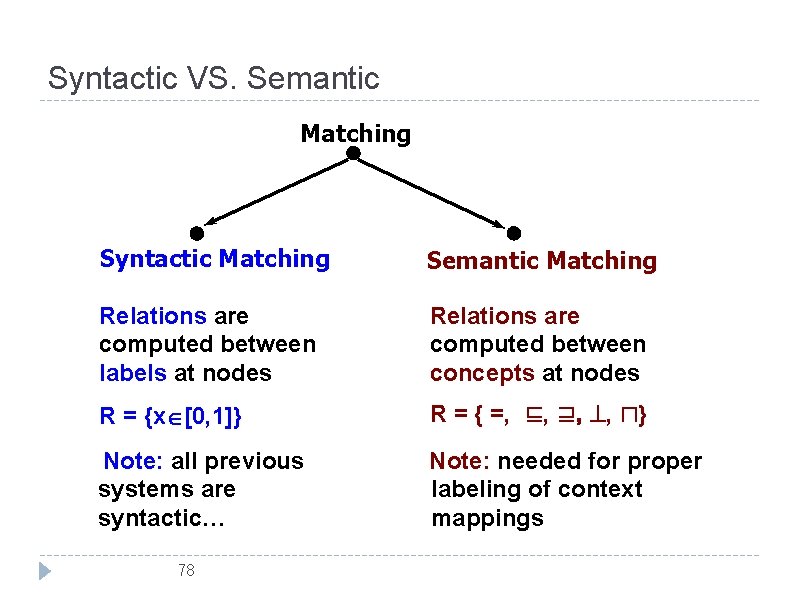
Syntactic VS. Semantic Matching Syntactic Matching Semantic Matching Relations are computed between labels at nodes Relations are computed between concepts at nodes R = {x [0, 1]} R = { =, ⊑, ⊒, , ⊓} Note: all previous systems are syntactic… Note: needed for proper labeling of context mappings 78

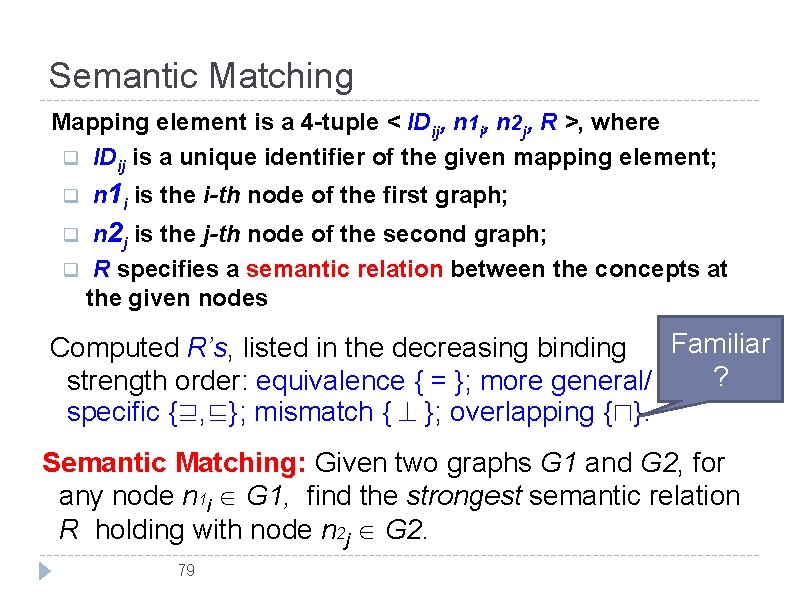
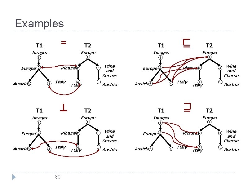
Semantic Matching Mapping element is a 4 -tuple < IDij, n 1 i, n 2 j, R >, where q IDij is a unique identifier of the given mapping element; q n 1 i is the i-th node of the first graph; n 2 j is the j-th node of the second graph; q R specifies a semantic relation between the concepts at the given nodes q Familiar Computed R’s, listed in the decreasing binding ? strength order: equivalence { = }; more general/ specific {⊒, ⊑}; mismatch { }; overlapping {⊓}. Semantic Matching: Given two graphs G 1 and G 2, for any node n 1 i G 1, find the strongest semantic relation R holding with node n 2 j G 2. 79

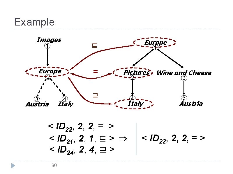
Example Images Europe ? = 2 4 3 Italy Austria Europe ? ⊑ 1 1 Pictures ⊒ ? < ID 22, 2, 2, = > < ID 21, 2, 1, ⊑ > < ID 24, 2, 4, ⊒ > 80 2 4 Italy Wine and Cheese 3 5 Austria < ID 22, 2, 2, = >

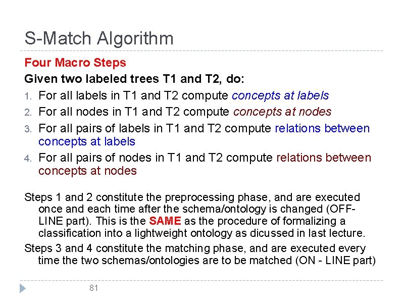
S-Match Algorithm Four Macro Steps Given two labeled trees T 1 and T 2, do: 1. For all labels in T 1 and T 2 compute concepts at labels 2. For all nodes in T 1 and T 2 compute concepts at nodes 3. For all pairs of labels in T 1 and T 2 compute relations between concepts at labels 4. For all pairs of nodes in T 1 and T 2 compute relations between concepts at nodes Steps 1 and 2 constitute the preprocessing phase, and are executed once and each time after the schema/ontology is changed (OFFLINE part). This is the SAME as the procedure of formalizing a classification into a lightweight ontology as dicussed in last lecture. Steps 3 and 4 constitute the matching phase, and are executed every time the two schemas/ontologies are to be matched (ON - LINE part) 81

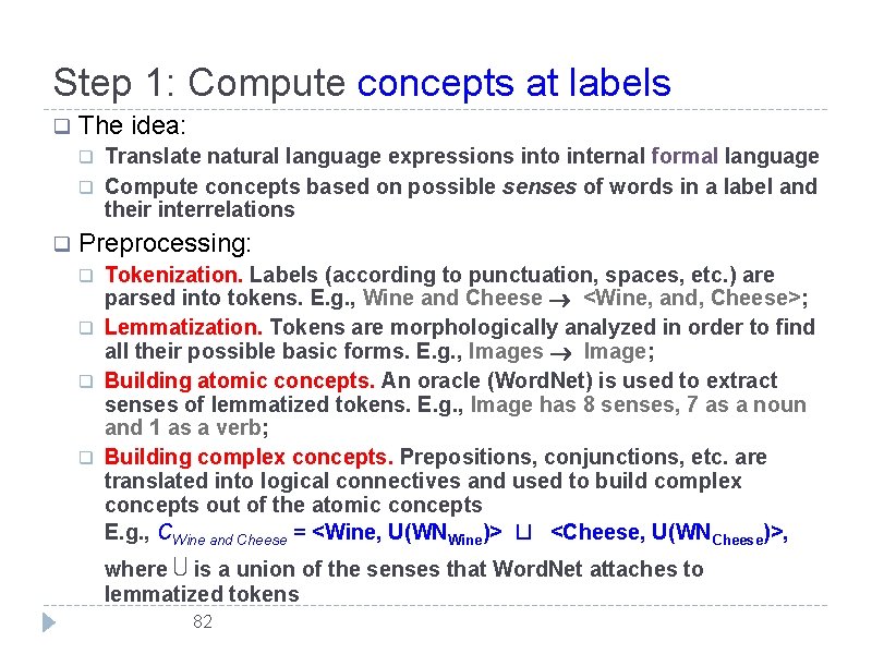
Step 1: Compute concepts at labels q The idea: q q q Translate natural language expressions into internal formal language Compute concepts based on possible senses of words in a label and their interrelations Preprocessing: q q Tokenization. Labels (according to punctuation, spaces, etc. ) are parsed into tokens. E. g. , Wine and Cheese <Wine, and, Cheese>; Lemmatization. Tokens are morphologically analyzed in order to find all their possible basic forms. E. g. , Images Image; Building atomic concepts. An oracle (Word. Net) is used to extract senses of lemmatized tokens. E. g. , Image has 8 senses, 7 as a noun and 1 as a verb; Building complex concepts. Prepositions, conjunctions, etc. are translated into logical connectives and used to build complex concepts out of the atomic concepts E. g. , CWine and Cheese = <Wine, U(WNWine)> ⊔ <Cheese, U(WNCheese)>, where ⋃ is a union of the senses that Word. Net attaches to lemmatized tokens 82

Step 2: Compute concepts at nodes The idea: extend concepts at labels by capturing the knowledge residing in a structure of a graph in order to define a context in which the given concept at a label occurs q Computation (basic case): Concept at a node for some node n is computed as an intersection of concepts at labels located above the given node, including the node itself q Europe 1 Pictures 2 4 Italy 3 Wine and Cheese 5 Austria C 4 = Ceurope ⊓CPictures⊓CItaly 83

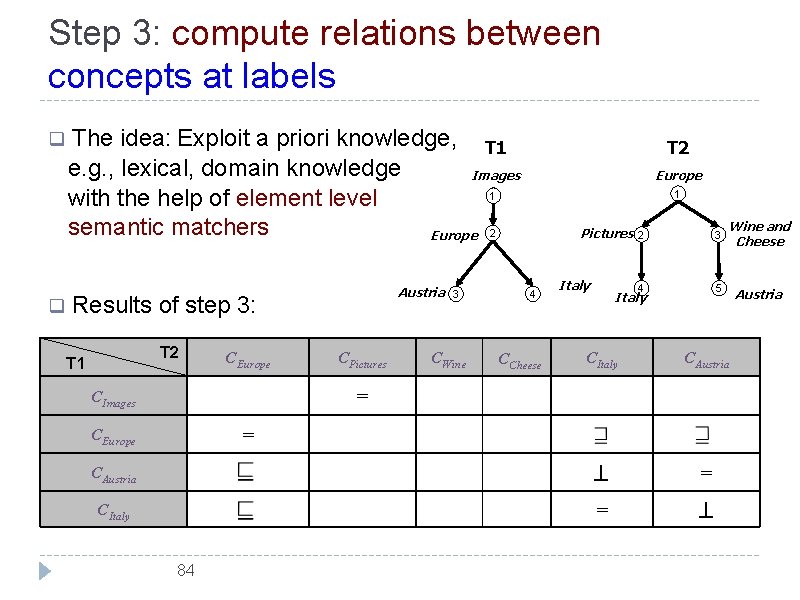
Step 3: compute relations between concepts at labels q q The idea: Exploit a priori knowledge, T 1 e. g. , lexical, domain knowledge Images 1 with the help of element level semantic matchers Europe 2 Austria Results of step 3: T 2 CPictures Europe 1 Pictures 4 Italy 2 3 4 5 Italy Wine and Cheese CItaly CAustria = CItaly = T 1 CEurope 3 T 2 CWine CCheese = CImages = CEurope 84 Austria

Don’t hurry to Step 4! q What we have done in Step 3? Find semantic relations. q What for? To build the semantic relation bases for further matching. q What is a ‘relation base’ in the logic sense? TBox! We are building the TBox! 85

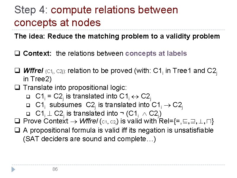
Step 4: compute relations between concepts at nodes The idea: Reduce the matching problem to a validity problem q Context: the relations between concepts at labels q Wffrel (C 1 i, C 2 j): relation to be proved (with: C 1 i in Tree 1 and C 2 j in Tree 2) q Translate into propositional logic: q C 1 i = C 2 j is translated into C 1 i C 2 j q C 1 i subsumes C 2 j is translated into C 1 i C 2 j q C 1 i C 2 j is translated into ¬ (C 1 i C 2 j) q Prove Context Wffrel (C 1 , C 2 ) is valid with Rel={=, ⊑, ⊒, ⊥, ⊓} q A propositional formula is valid iff its negation is unsatisfiable (SAT deciders are sound and complete…) i 86 j

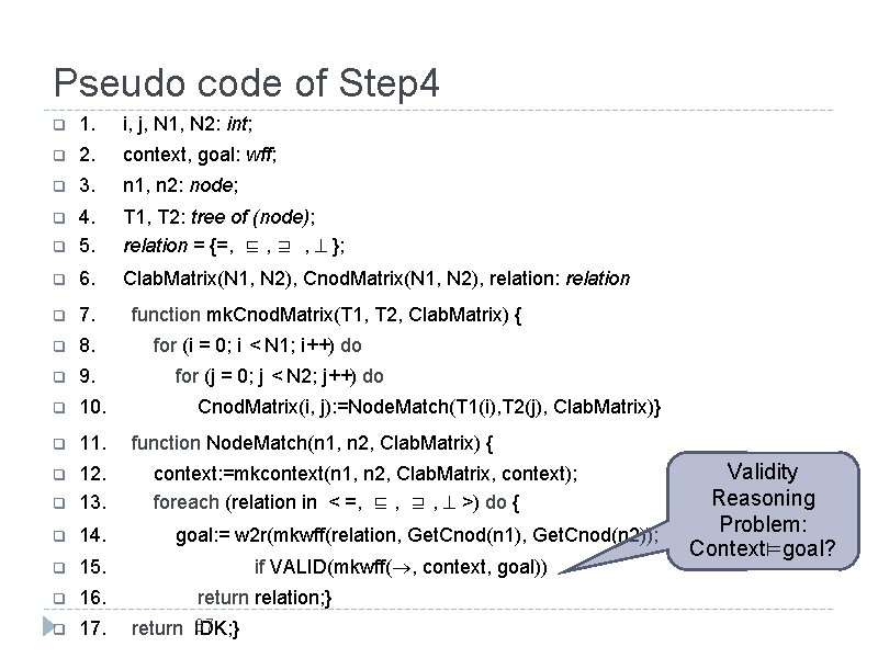
Pseudo code of Step 4 q 1. i, j, N 1, N 2: int; q 2. context, goal: wff; q 3. n 1, n 2: node; q q 4. 5. T 1, T 2: tree of (node); relation = {=, ⊑ , ⊒ , }; q 6. Clab. Matrix(N 1, N 2), Cnod. Matrix(N 1, N 2), relation: relation q 7. q 8. q 9. q 10. q 11. q q 12. 13. q 14. q 15. q 16. q 17. function mk. Cnod. Matrix(T 1, T 2, Clab. Matrix) { for (i = 0; i < N 1; i++) do for (j = 0; j < N 2; j++) do Cnod. Matrix(i, j): =Node. Match(T 1(i), T 2(j), Clab. Matrix)} function Node. Match(n 1, n 2, Clab. Matrix) { context: =mkcontext(n 1, n 2, Clab. Matrix, context); foreach (relation in < =, ⊑ , ⊒ , >) do { goal: = w 2 r(mkwff(relation, Get. Cnod(n 1), Get. Cnod(n 2)); if VALID(mkwff( , context, goal)) return relation; } 87 return IDK; } Validity Reasoning Problem: Context⊨goal?

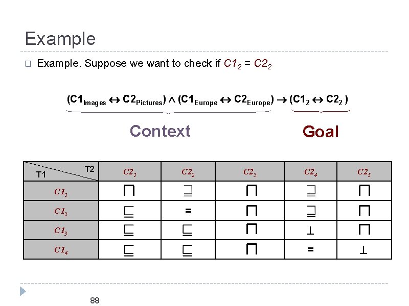
Example q Example. Suppose we want to check if C 12 = C 22 (C 1 Images C 2 Pictures) (C 1 Europe C 2 Europe) (C 12 C 22 ) Context T 2 T 1 C 22 Goal C 23 C 24 C 25 C 11 = C 12 C 13 C 14 = 88

Examples = T 1 T 2 Images Europe 1 1 Europe Pictures 2 2 Austria 3 4 4 5 Italy T 1 Wine and Cheese Austria Europe Pictures 2 2 Austria 3 4 Italy 3 4 5 Italy T 2 T 1 T 2 Images Europe 1 1 Europe Austria 3 Italy 3 Pictures 2 2 4 Italy 89 4 Italy 3 5 Wine and Cheese Austria Europe Austria 3 Pictures 2 2 4 Italy 3 5 Wine and Cheese Austria

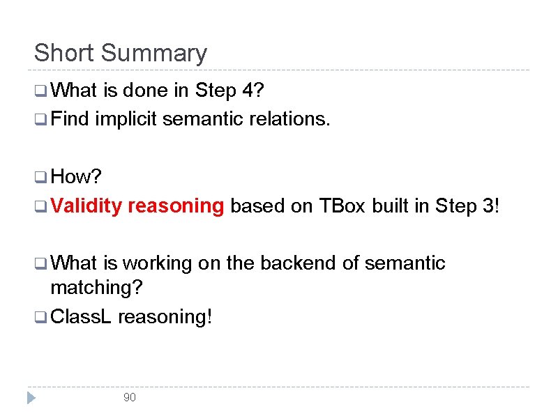
Short Summary q What is done in Step 4? q Find implicit semantic relations. q How? q Validity reasoning based on TBox built in Step 3! q What is working on the backend of semantic matching? q Class. L reasoning! 90

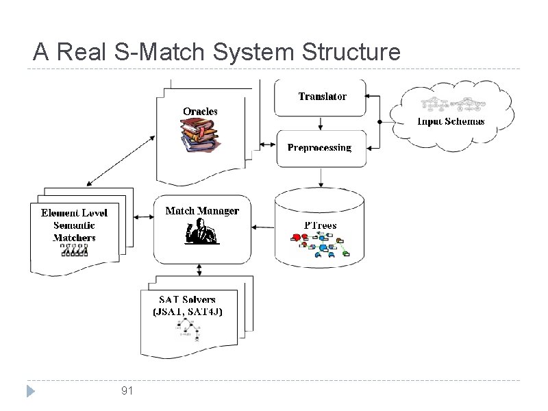
A Real S-Match System Structure 91

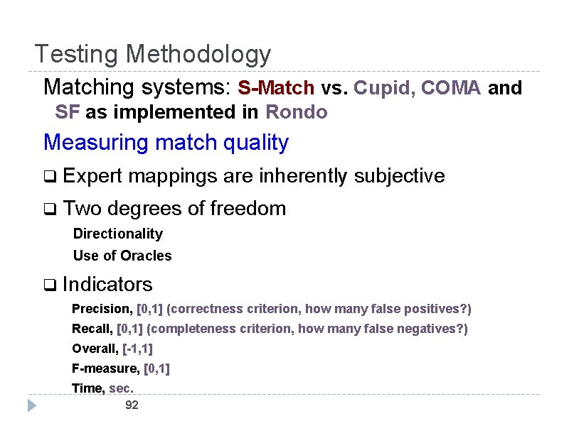
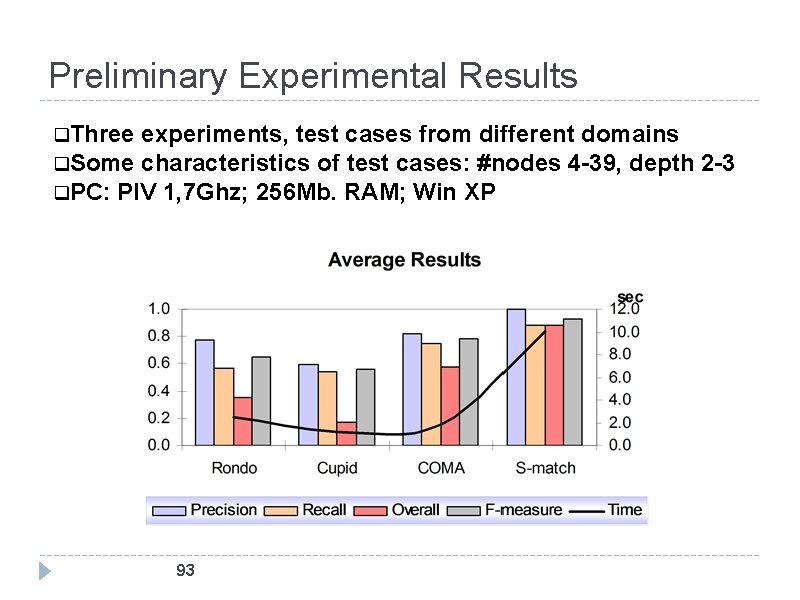
Testing Methodology Matching systems: S-Match vs. Cupid, COMA and SF as implemented in Rondo Measuring match quality q Expert mappings are inherently subjective q Two degrees of freedom Directionality Use of Oracles q Indicators Precision, [0, 1] (correctness criterion, how many false positives? ) Recall, [0, 1] (completeness criterion, how many false negatives? ) Overall, [-1, 1] F-measure, [0, 1] Time, sec. 92

Preliminary Experimental Results q. Three experiments, test cases from different domains q. Some characteristics of test cases: #nodes 4 -39, depth 2 -3 q. PC: PIV 1, 7 Ghz; 256 Mb. RAM; Win XP 93

References & Credits q References: F. Giunchiglia, P. Shvaiko, “Semantic matching. ” Knowledge Engineering Review, 18(3): 265 -280, 2003. F. Giunchiglia, M. Marchese, I. Zaihrayeu. “Encoding Classifications into Lightweight Ontologies. ” J. of Data Semantics VIII, Springer-Verlag LNCS 4380, pp 57 -81, 2007. F. Giunchiglia, I. Zaihrayeu. “Lightweight Ontologies” Encyclopedia of Database Systems , Springer-Verlag, 2008. Available as a DIT Technical Report here. 94