Chapter 13 Output Stages and Power Amplifiers 13

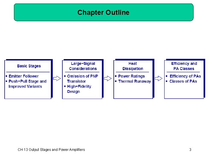
Chapter 13 Output Stages and Power Amplifiers Ø Ø Ø Ø Ø 13. 1 13. 2 13. 3 13. 4 13. 5 13. 6 13. 7 13. 8 13. 9 General Considerations Emitter Follower as Power Amplifier Push-Pull Stage Improved Push-Pull Stage Large-Signal Considerations Short Circuit Protection Heat Dissipation Efficiency Power Amplifier Classes 1

Why Power Amplifiers? Ø Drive a load with high power. Ø Cell phone needs 1 W of power at the antenna. Ø Audio system needs tens to hundreds Watts of power. Ø Ordinary Voltage/Current amplifiers are not equipped for such applications CH 13 Output Stages and Power Amplifiers 2

Chapter Outline CH 13 Output Stages and Power Amplifiers 3

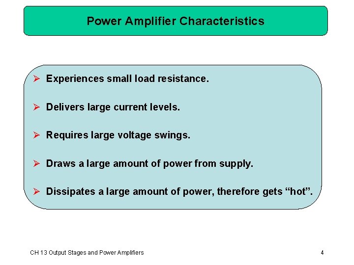
Power Amplifier Characteristics Ø Experiences small load resistance. Ø Delivers large current levels. Ø Requires large voltage swings. Ø Draws a large amount of power from supply. Ø Dissipates a large amount of power, therefore gets “hot”. CH 13 Output Stages and Power Amplifiers 4

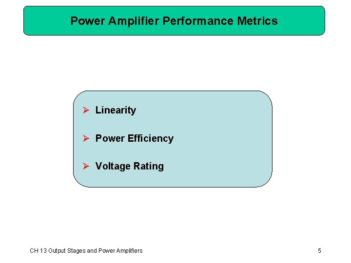
Power Amplifier Performance Metrics Ø Linearity Ø Power Efficiency Ø Voltage Rating CH 13 Output Stages and Power Amplifiers 5

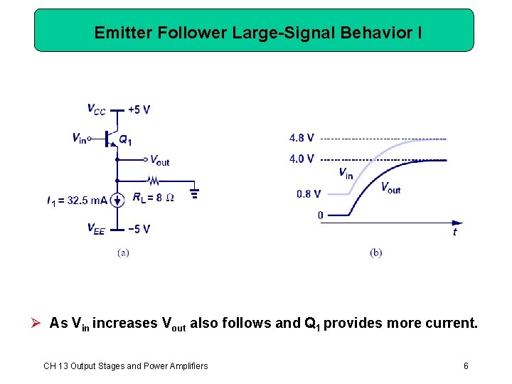
Emitter Follower Large-Signal Behavior I Ø As Vin increases Vout also follows and Q 1 provides more current. CH 13 Output Stages and Power Amplifiers 6

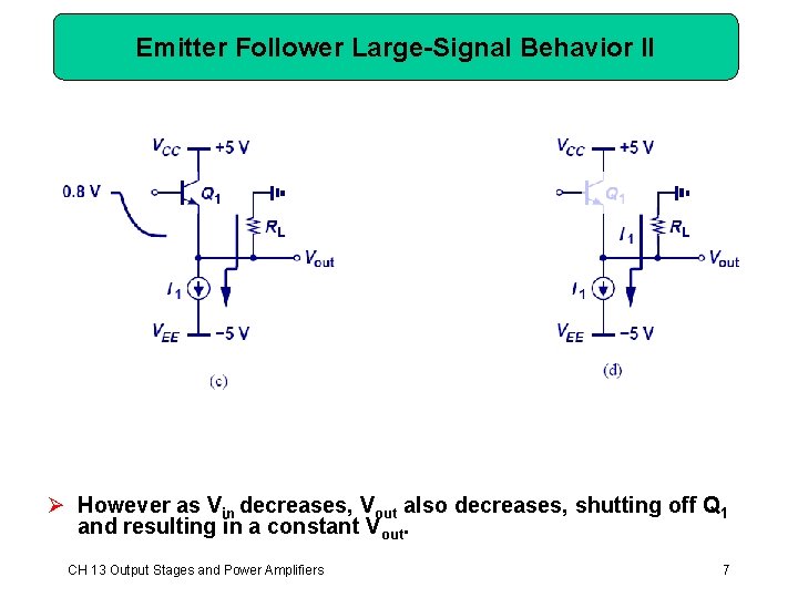
Emitter Follower Large-Signal Behavior II Ø However as Vin decreases, Vout also decreases, shutting off Q 1 and resulting in a constant Vout. CH 13 Output Stages and Power Amplifiers 7

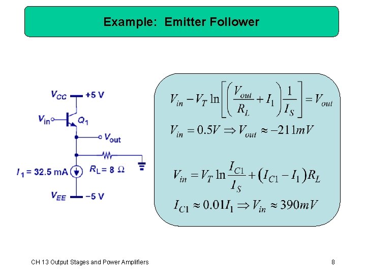
Example: Emitter Follower CH 13 Output Stages and Power Amplifiers 8

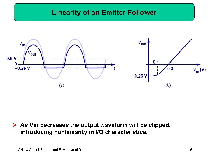
Linearity of an Emitter Follower Ø As Vin decreases the output waveform will be clipped, introducing nonlinearity in I/O characteristics. CH 13 Output Stages and Power Amplifiers 9

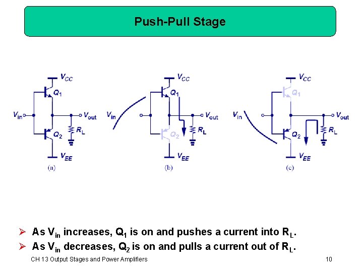
Push-Pull Stage Ø As Vin increases, Q 1 is on and pushes a current into RL. Ø As Vin decreases, Q 2 is on and pulls a current out of RL. CH 13 Output Stages and Power Amplifiers 10

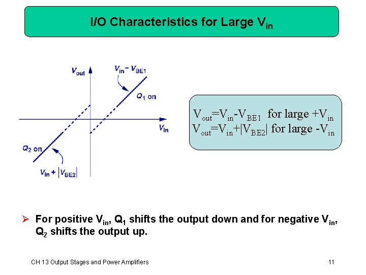
I/O Characteristics for Large Vin Vout=Vin-VBE 1 for large +Vin Vout=Vin+|VBE 2| for large -Vin Ø For positive Vin, Q 1 shifts the output down and for negative Vin, Q 2 shifts the output up. CH 13 Output Stages and Power Amplifiers 11

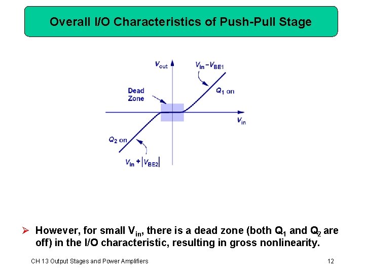
Overall I/O Characteristics of Push-Pull Stage Ø However, for small Vin, there is a dead zone (both Q 1 and Q 2 are off) in the I/O characteristic, resulting in gross nonlinearity. CH 13 Output Stages and Power Amplifiers 12

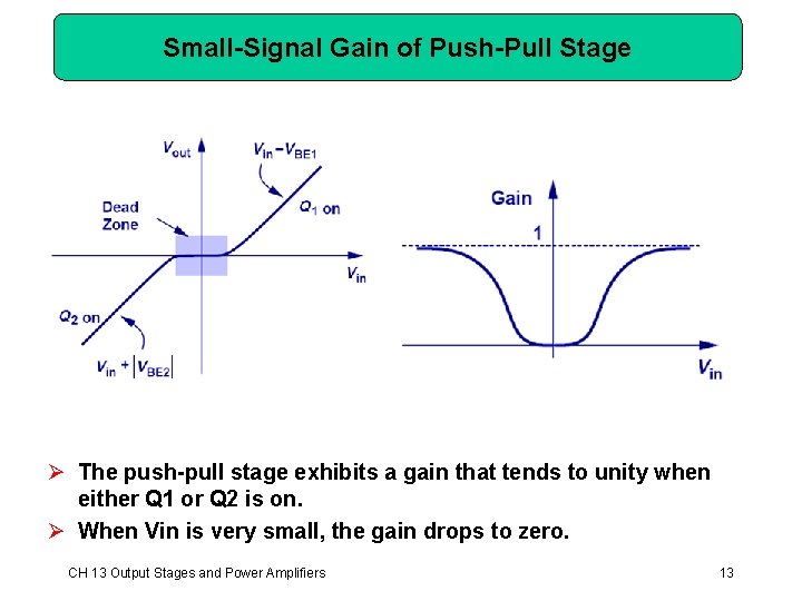
Small-Signal Gain of Push-Pull Stage Ø The push-pull stage exhibits a gain that tends to unity when either Q 1 or Q 2 is on. Ø When Vin is very small, the gain drops to zero. CH 13 Output Stages and Power Amplifiers 13

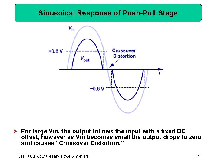
Sinusoidal Response of Push-Pull Stage Ø For large Vin, the output follows the input with a fixed DC offset, however as Vin becomes small the output drops to zero and causes “Crossover Distortion. ” CH 13 Output Stages and Power Amplifiers 14

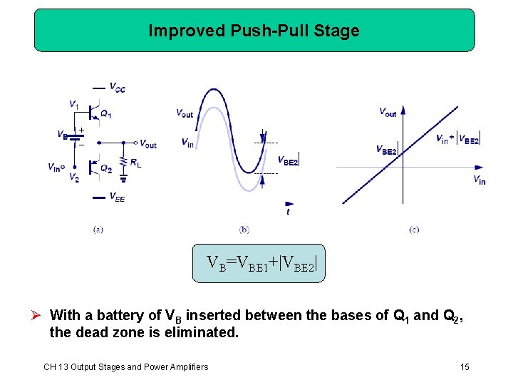
Improved Push-Pull Stage VB=VBE 1+|VBE 2| Ø With a battery of VB inserted between the bases of Q 1 and Q 2, the dead zone is eliminated. CH 13 Output Stages and Power Amplifiers 15

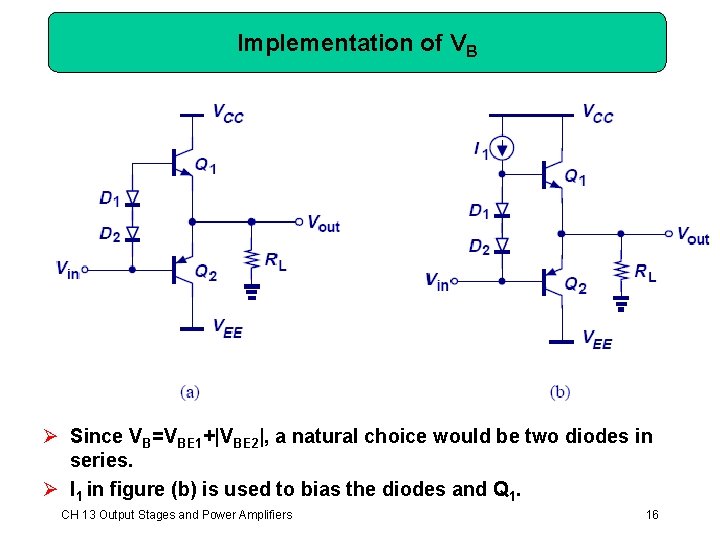
Implementation of VB Ø Since VB=VBE 1+|VBE 2|, a natural choice would be two diodes in series. Ø I 1 in figure (b) is used to bias the diodes and Q 1. CH 13 Output Stages and Power Amplifiers 16

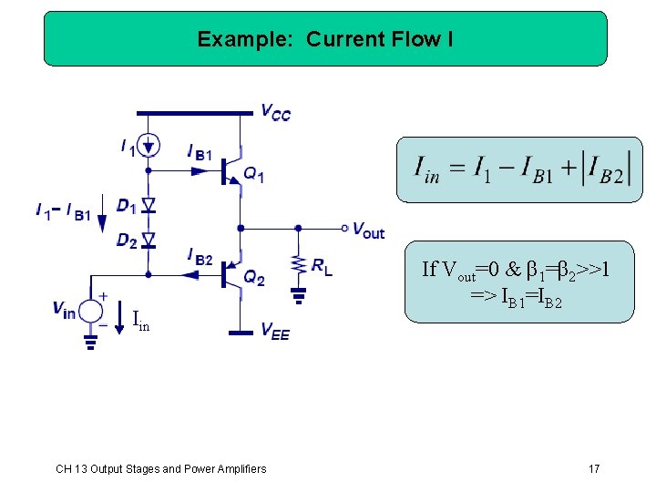
Example: Current Flow I Iin CH 13 Output Stages and Power Amplifiers If Vout=0 & β 1=β 2>>1 => IB 1=IB 2 17

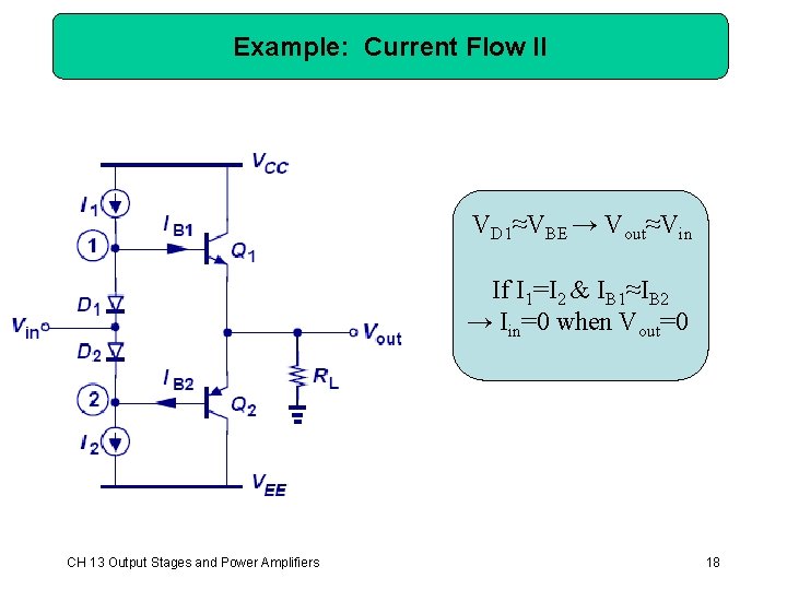
Example: Current Flow II VD 1≈VBE → Vout≈Vin If I 1=I 2 & IB 1≈IB 2 → Iin=0 when Vout=0 CH 13 Output Stages and Power Amplifiers 18

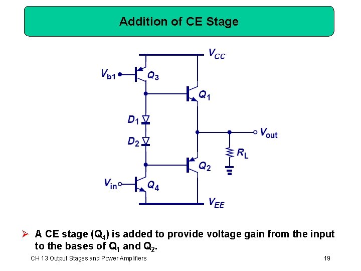
Addition of CE Stage Ø A CE stage (Q 4) is added to provide voltage gain from the input to the bases of Q 1 and Q 2. CH 13 Output Stages and Power Amplifiers 19

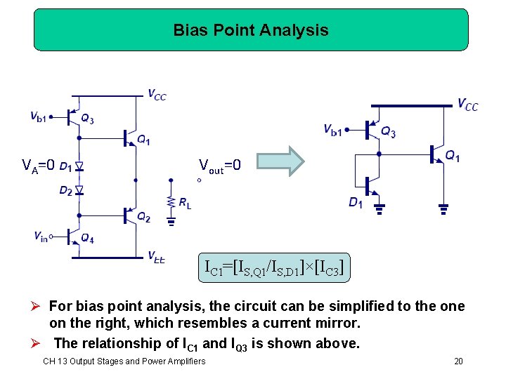
Bias Point Analysis VA=0 Vout=0 IC 1=[IS, Q 1/IS, D 1]×[IC 3] Ø For bias point analysis, the circuit can be simplified to the on the right, which resembles a current mirror. Ø The relationship of IC 1 and IQ 3 is shown above. CH 13 Output Stages and Power Amplifiers 20

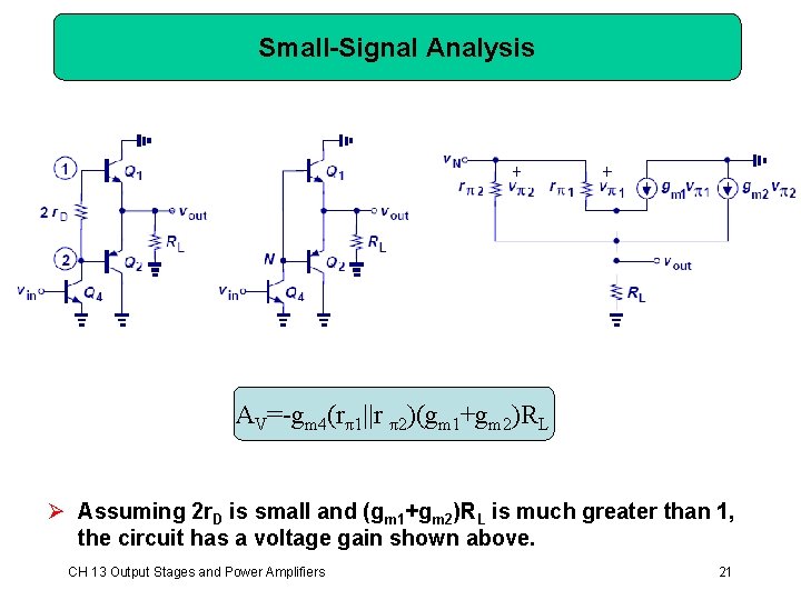
Small-Signal Analysis AV=-gm 4(rπ1||r π2)(gm 1+gm 2)RL Ø Assuming 2 r. D is small and (gm 1+gm 2)RL is much greater than 1, the circuit has a voltage gain shown above. CH 13 Output Stages and Power Amplifiers 21

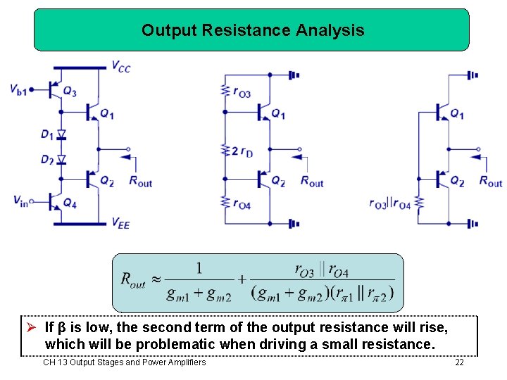
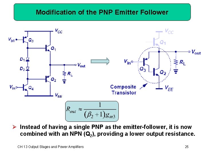
Output Resistance Analysis Ø If β is low, the second term of the output resistance will rise, which will be problematic when driving a small resistance. CH 13 Output Stages and Power Amplifiers 22

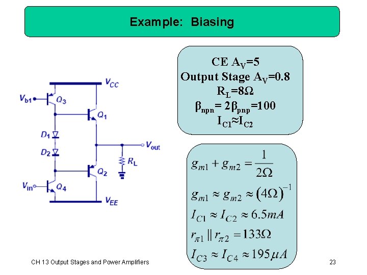
Example: Biasing CE AV=5 Output Stage AV=0. 8 RL=8Ω βnpn= 2βpnp=100 IC 1≈IC 2 CH 13 Output Stages and Power Amplifiers 23

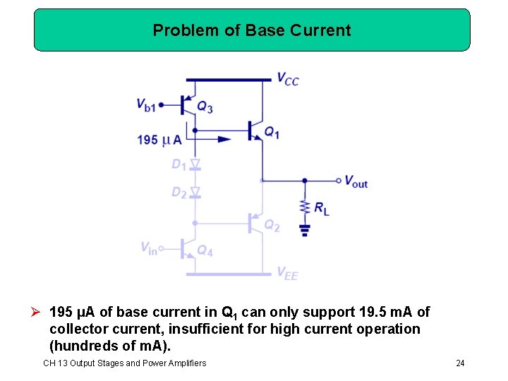
Problem of Base Current Ø 195 µA of base current in Q 1 can only support 19. 5 m. A of collector current, insufficient for high current operation (hundreds of m. A). CH 13 Output Stages and Power Amplifiers 24

Modification of the PNP Emitter Follower Ø Instead of having a single PNP as the emitter-follower, it is now combined with an NPN (Q 2), providing a lower output resistance. CH 13 Output Stages and Power Amplifiers 25

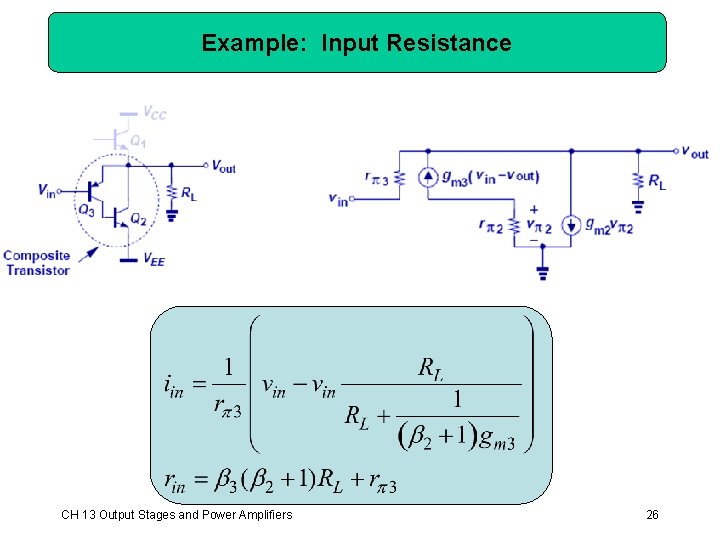
Example: Input Resistance CH 13 Output Stages and Power Amplifiers 26

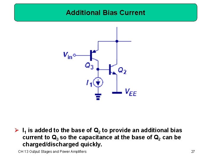
Additional Bias Current Ø I 1 is added to the base of Q 2 to provide an additional bias current to Q 3 so the capacitance at the base of Q 2 can be charged/discharged quickly. CH 13 Output Stages and Power Amplifiers 27

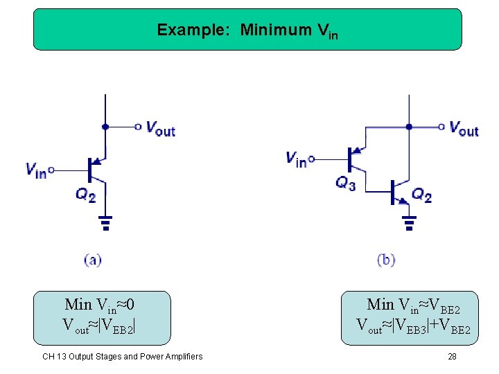
Example: Minimum Vin Min Vin≈0 Vout≈|VEB 2| CH 13 Output Stages and Power Amplifiers Min Vin≈VBE 2 Vout≈|VEB 3|+VBE 2 28

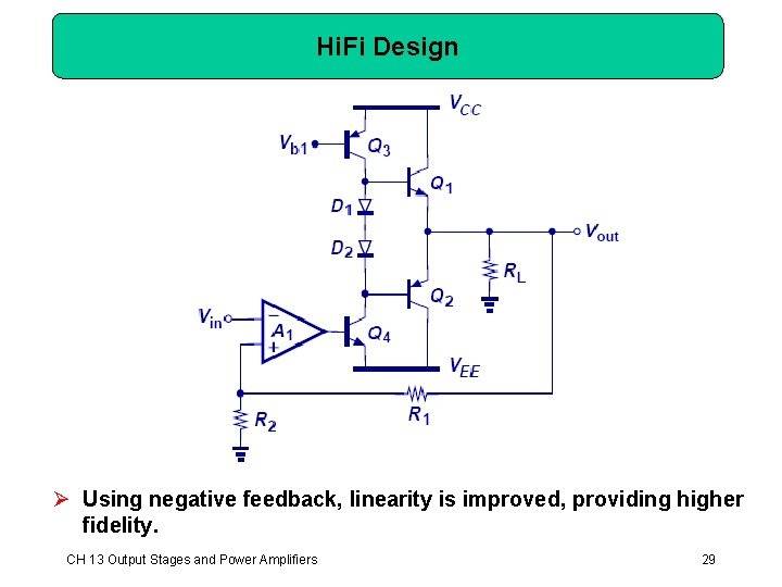
Hi. Fi Design Ø Using negative feedback, linearity is improved, providing higher fidelity. CH 13 Output Stages and Power Amplifiers 29

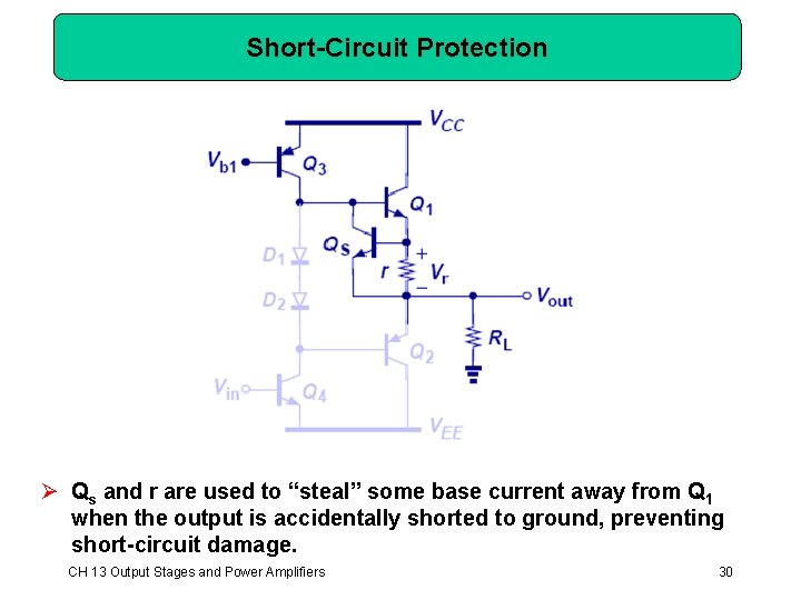
Short-Circuit Protection Ø Qs and r are used to “steal” some base current away from Q 1 when the output is accidentally shorted to ground, preventing short-circuit damage. CH 13 Output Stages and Power Amplifiers 30

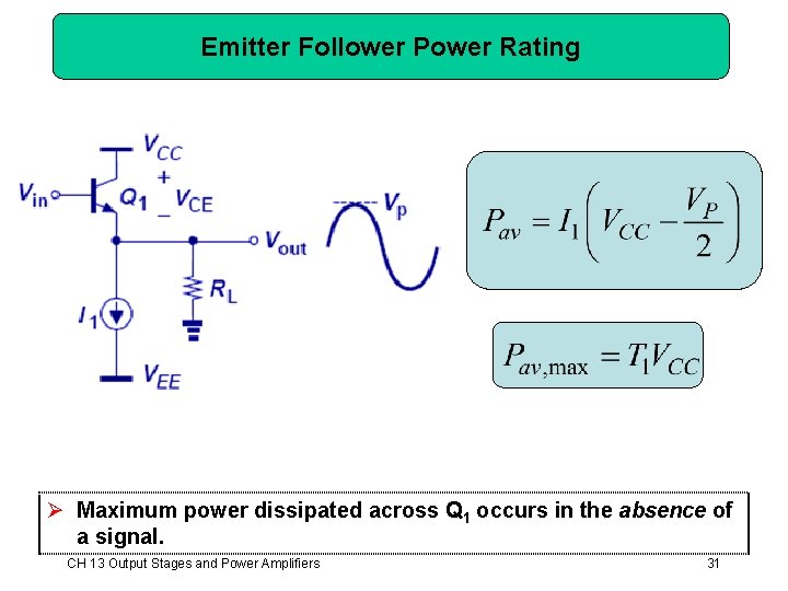
Emitter Follower Power Rating Ø Maximum power dissipated across Q 1 occurs in the absence of a signal. CH 13 Output Stages and Power Amplifiers 31

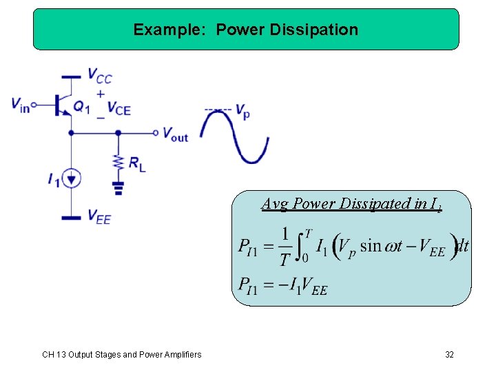
Example: Power Dissipation Avg Power Dissipated in I 1 CH 13 Output Stages and Power Amplifiers 32

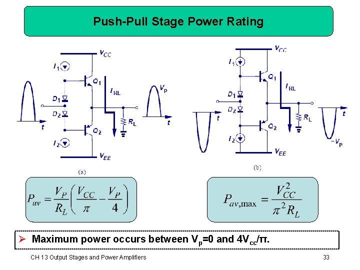
Push-Pull Stage Power Rating Ø Maximum power occurs between Vp=0 and 4 Vcc/π. CH 13 Output Stages and Power Amplifiers 33

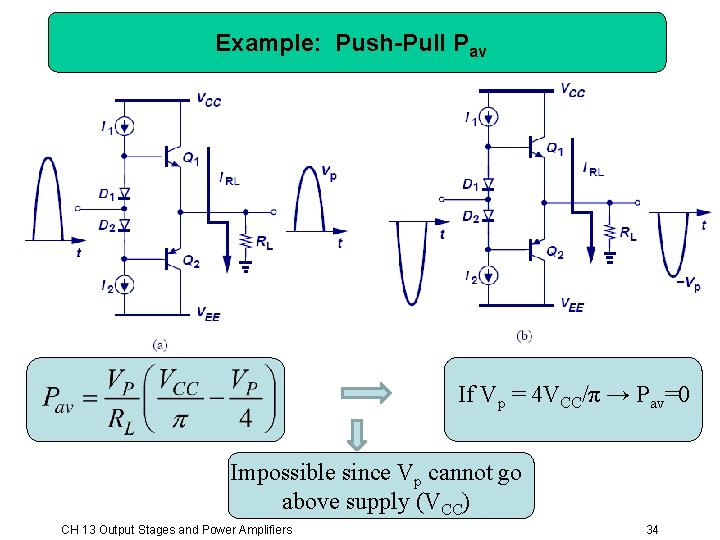
Example: Push-Pull Pav If Vp = 4 VCC/π → Pav=0 Impossible since Vp cannot go above supply (VCC) CH 13 Output Stages and Power Amplifiers 34

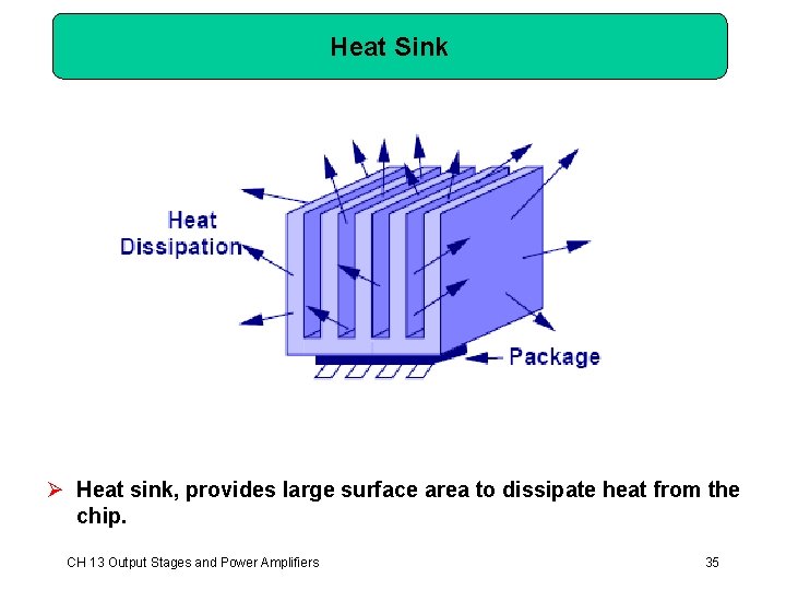
Heat Sink Ø Heat sink, provides large surface area to dissipate heat from the chip. CH 13 Output Stages and Power Amplifiers 35

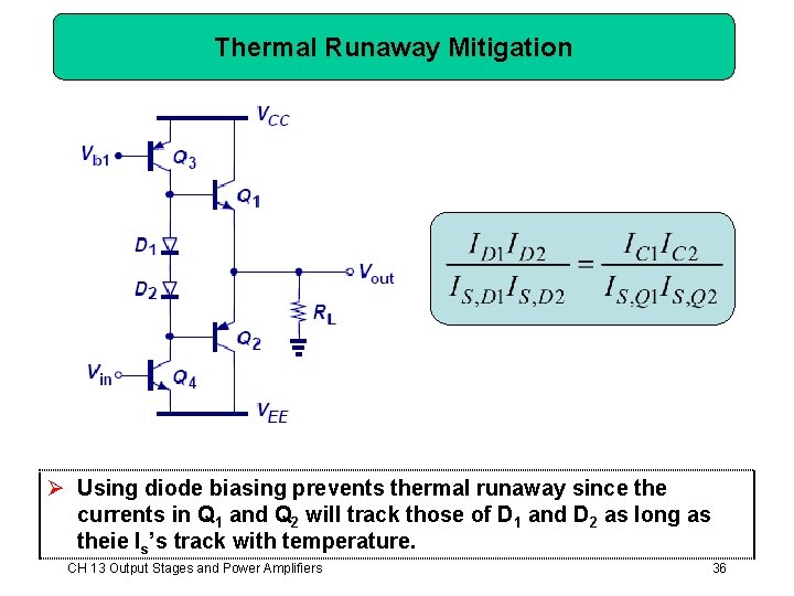
Thermal Runaway Mitigation Ø Using diode biasing prevents thermal runaway since the currents in Q 1 and Q 2 will track those of D 1 and D 2 as long as theie Is’s track with temperature. CH 13 Output Stages and Power Amplifiers 36

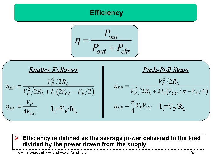
Efficiency Emitter Follower I 1=VP/RL Push-Pull Stage I 1=VP/RL Ø Efficiency is defined as the average power delivered to the load divided by the power drawn from the supply CH 13 Output Stages and Power Amplifiers 37

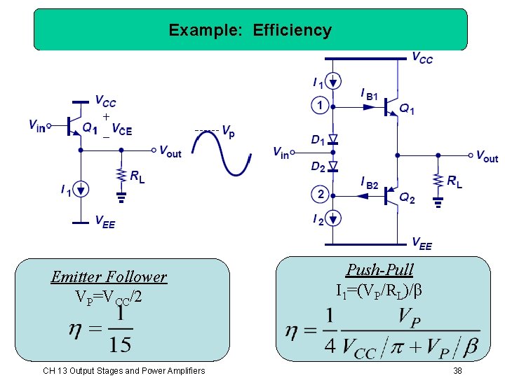
Example: Efficiency Emitter Follower VP=VCC/2 CH 13 Output Stages and Power Amplifiers Push-Pull I 1=(VP/RL)/β 38

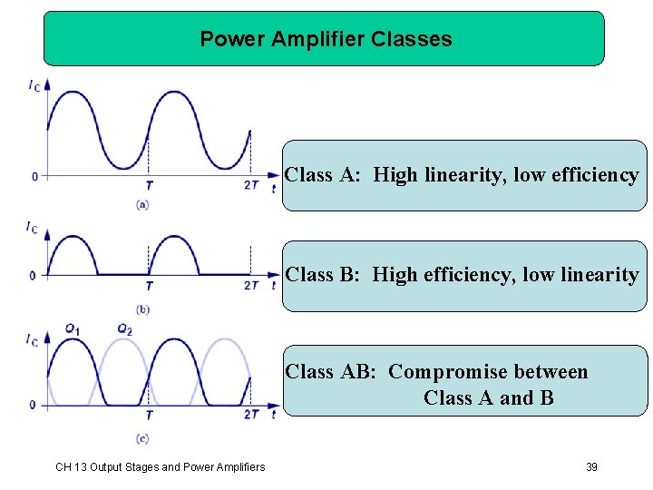
Power Amplifier Classes Class A: High linearity, low efficiency Class B: High efficiency, low linearity Class AB: Compromise between Class A and B CH 13 Output Stages and Power Amplifiers 39

Chapter 14 Analog Filters Ø Ø Ø 14. 1 14. 2 14. 3 14. 4 14. 5 General Considerations First-Order Filters Second-Order Filters Active Filters Approximation of Filter Response 40

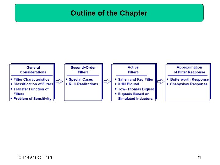
Outline of the Chapter CH 14 Analog Filters 41

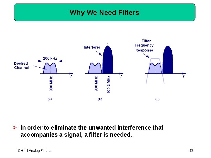
Why We Need Filters Ø In order to eliminate the unwanted interference that accompanies a signal, a filter is needed. CH 14 Analog Filters 42

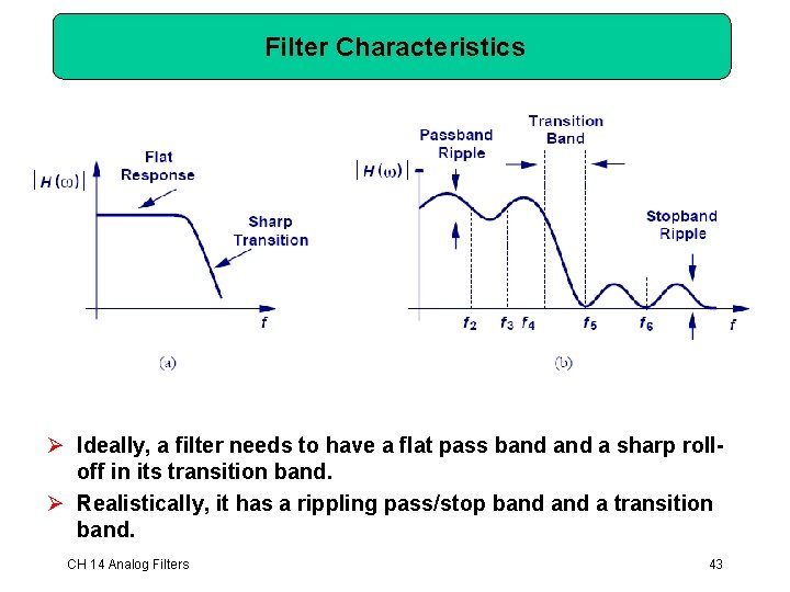
Filter Characteristics Ø Ideally, a filter needs to have a flat pass band a sharp rolloff in its transition band. Ø Realistically, it has a rippling pass/stop band a transition band. CH 14 Analog Filters 43

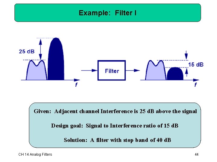
Example: Filter I Given: Adjacent channel Interference is 25 d. B above the signal Design goal: Signal to Interference ratio of 15 d. B Solution: A filter with stop band of 40 d. B CH 14 Analog Filters 44

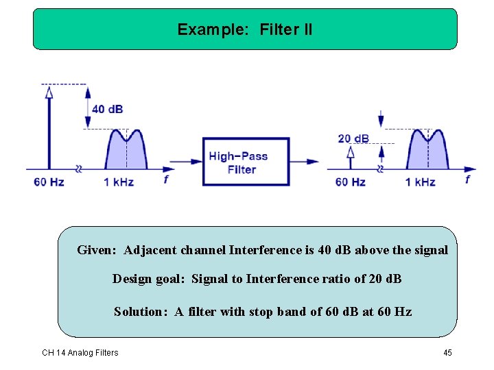
Example: Filter II Given: Adjacent channel Interference is 40 d. B above the signal Design goal: Signal to Interference ratio of 20 d. B Solution: A filter with stop band of 60 d. B at 60 Hz CH 14 Analog Filters 45

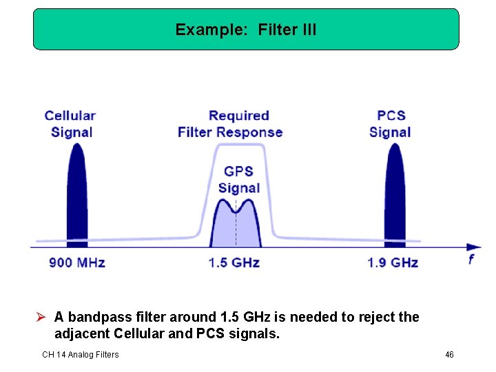
Example: Filter III Ø A bandpass filter around 1. 5 GHz is needed to reject the adjacent Cellular and PCS signals. CH 14 Analog Filters 46

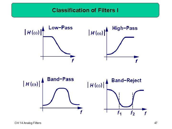
Classification of Filters I CH 14 Analog Filters 47

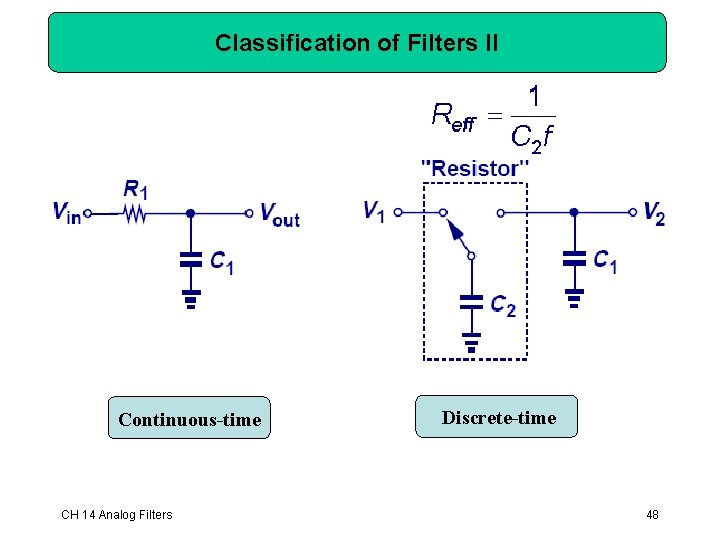
Classification of Filters II Continuous-time CH 14 Analog Filters Discrete-time 48

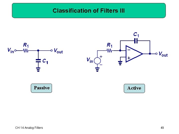
Classification of Filters III Passive CH 14 Analog Filters Active 49

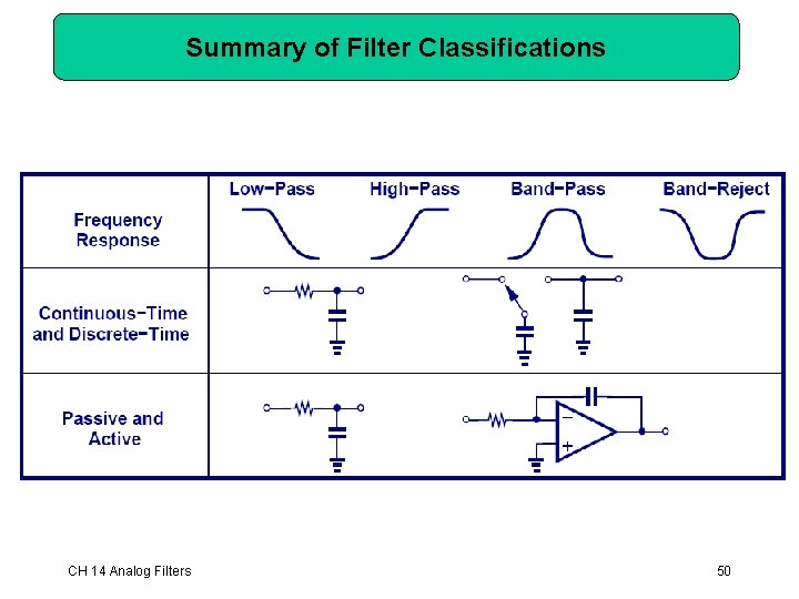
Summary of Filter Classifications CH 14 Analog Filters 50

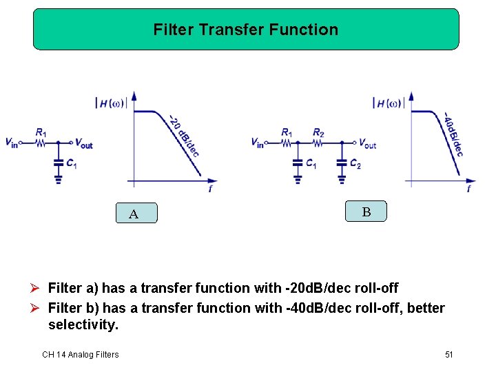
Filter Transfer Function A B Ø Filter a) has a transfer function with -20 d. B/dec roll-off Ø Filter b) has a transfer function with -40 d. B/dec roll-off, better selectivity. CH 14 Analog Filters 51

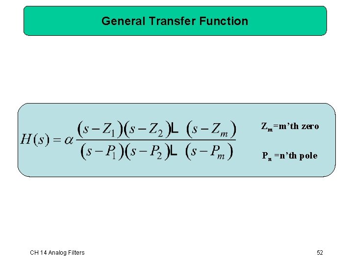
General Transfer Function Zm=m’th zero Pn =n’th pole CH 14 Analog Filters 52

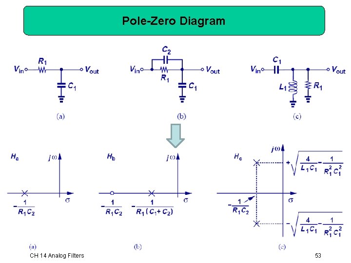
Pole-Zero Diagram CH 14 Analog Filters 53

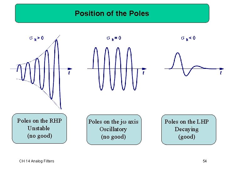
Position of the Poles on the RHP Unstable (no good) CH 14 Analog Filters Poles on the jω axis Oscillatory (no good) Poles on the LHP Decaying (good) 54

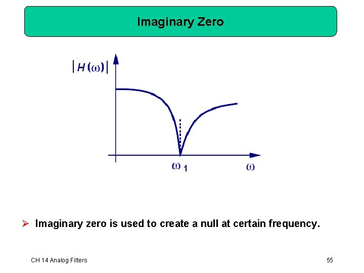
Imaginary Zero Ø Imaginary zero is used to create a null at certain frequency. CH 14 Analog Filters 55

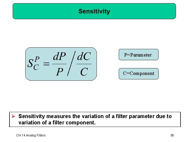
Sensitivity P=Parameter C=Component Ø Sensitivity measures the variation of a filter parameter due to variation of a filter component. CH 14 Analog Filters 56

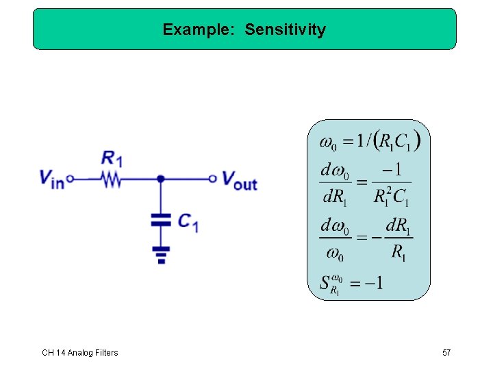
Example: Sensitivity CH 14 Analog Filters 57

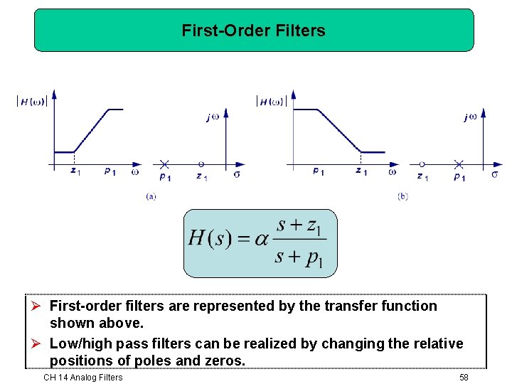
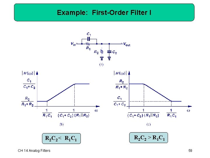
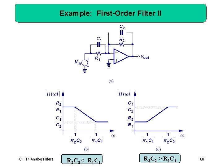
First-Order Filters Ø First-order filters are represented by the transfer function shown above. Ø Low/high pass filters can be realized by changing the relative positions of poles and zeros. CH 14 Analog Filters 58

Example: First-Order Filter I R 2 C 2 < R 1 CH 14 Analog Filters R 2 C 2 > R 1 C 1 59

Example: First-Order Filter II CH 14 Analog Filters R 2 C 2 < R 1 C 1 R 2 C 2 > R 1 C 1 60

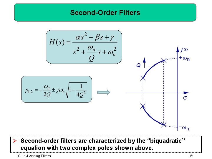
Second-Order Filters Ø Second-order filters are characterized by the “biquadratic” equation with two complex poles shown above. CH 14 Analog Filters 61

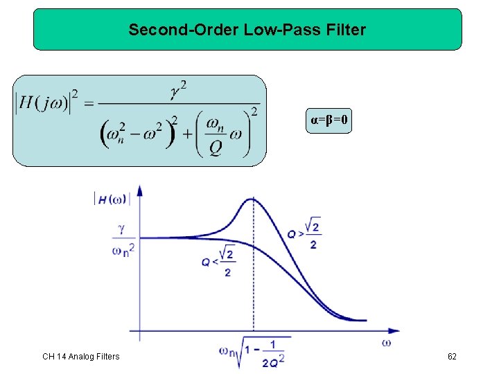
Second-Order Low-Pass Filter α=β=0 CH 14 Analog Filters 62

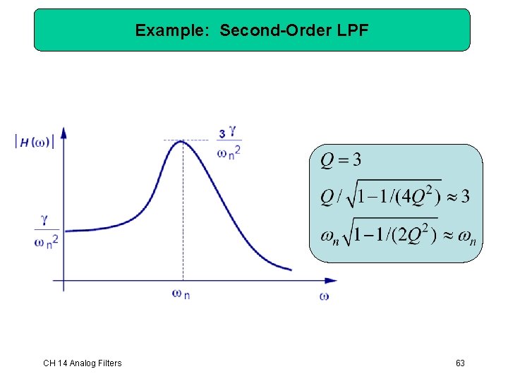
Example: Second-Order LPF CH 14 Analog Filters 63

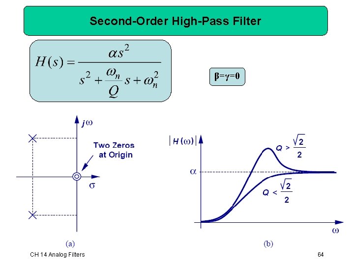
Second-Order High-Pass Filter β=γ=0 CH 14 Analog Filters 64

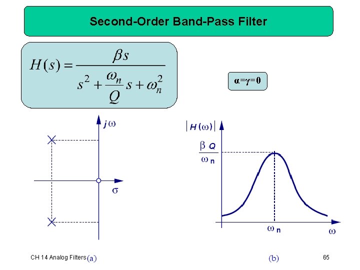
Second-Order Band-Pass Filter α=γ=0 CH 14 Analog Filters 65

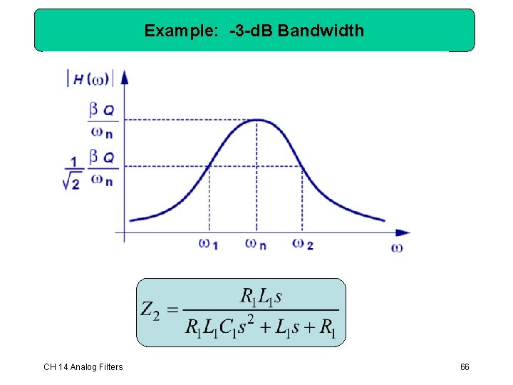
Example: -3 -d. B Bandwidth CH 14 Analog Filters 66

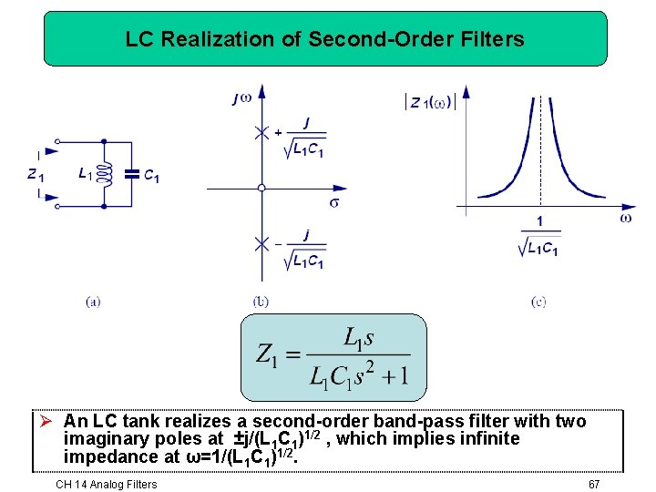
LC Realization of Second-Order Filters Ø An LC tank realizes a second-order band-pass filter with two imaginary poles at ±j/(L 1 C 1)1/2 , which implies infinite impedance at ω=1/(L 1 C 1)1/2. CH 14 Analog Filters 67

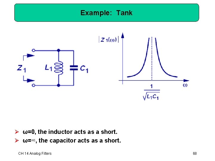
Example: Tank Ø ω=0, the inductor acts as a short. Ø ω=∞, the capacitor acts as a short. CH 14 Analog Filters 68

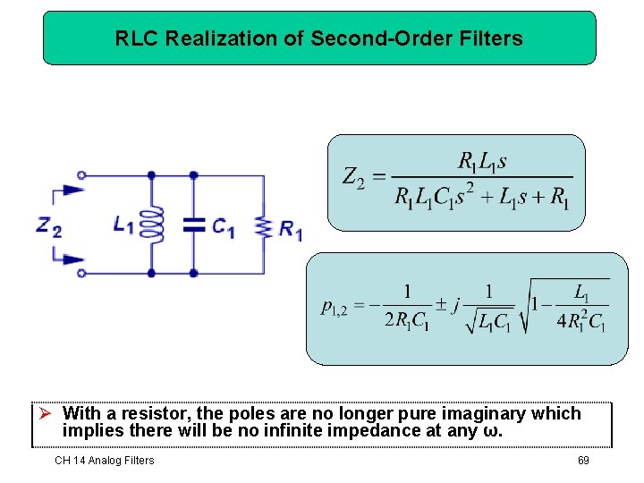
RLC Realization of Second-Order Filters Ø With a resistor, the poles are no longer pure imaginary which implies there will be no infinite impedance at any ω. CH 14 Analog Filters 69

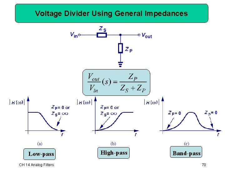
Voltage Divider Using General Impedances Low-pass CH 14 Analog Filters High-pass Band-pass 70

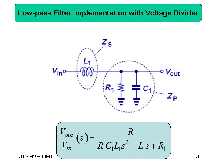
Low-pass Filter Implementation with Voltage Divider CH 14 Analog Filters 71

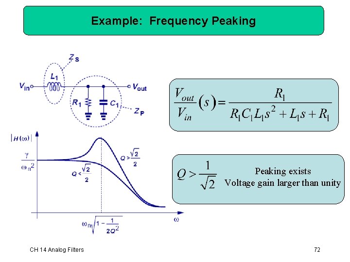
Example: Frequency Peaking exists Voltage gain larger than unity CH 14 Analog Filters 72

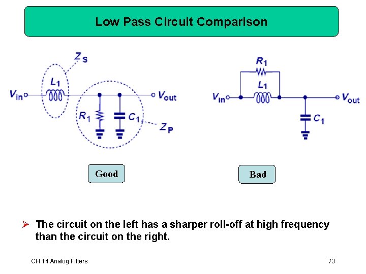
Low Pass Circuit Comparison Good Bad Ø The circuit on the left has a sharper roll-off at high frequency than the circuit on the right. CH 14 Analog Filters 73

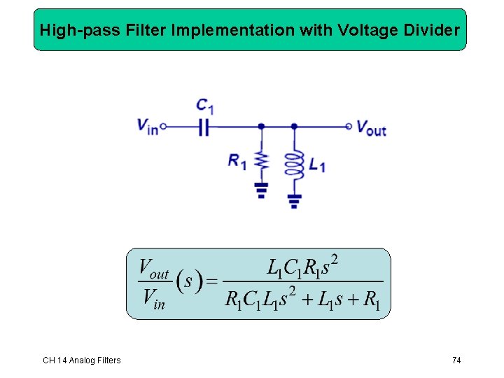
High-pass Filter Implementation with Voltage Divider CH 14 Analog Filters 74

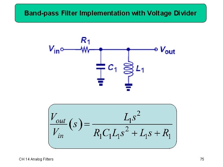
Band-pass Filter Implementation with Voltage Divider CH 14 Analog Filters 75

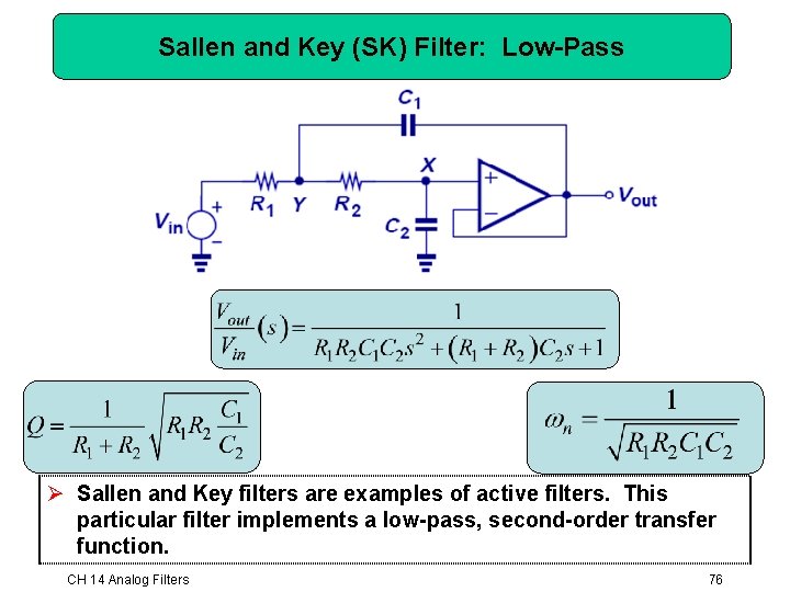
Sallen and Key (SK) Filter: Low-Pass Ø Sallen and Key filters are examples of active filters. This particular filter implements a low-pass, second-order transfer function. CH 14 Analog Filters 76

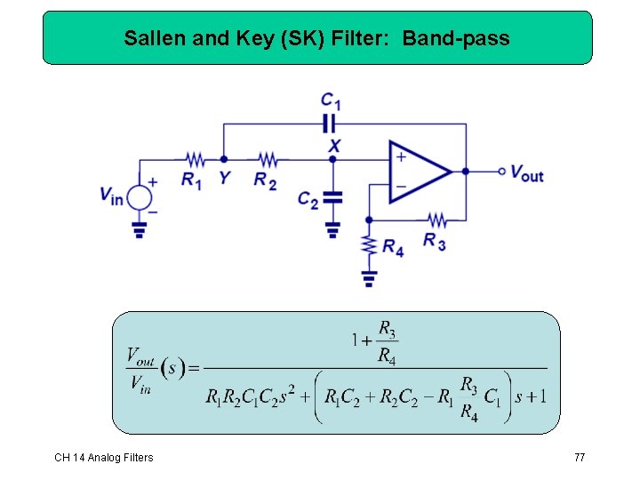
Sallen and Key (SK) Filter: Band-pass CH 14 Analog Filters 77

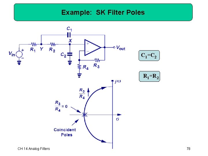
Example: SK Filter Poles C 1=C 2 R 1=R 2 CH 14 Analog Filters 78

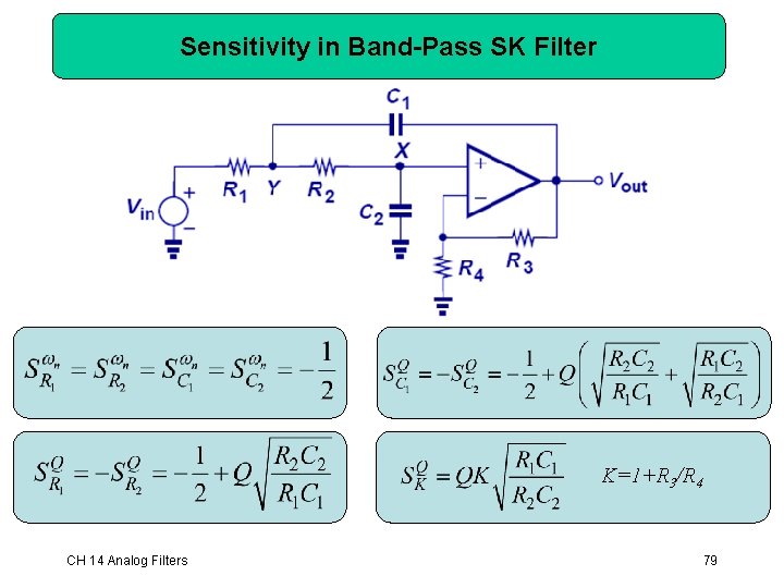
Sensitivity in Band-Pass SK Filter K=1+R 3/R 4 CH 14 Analog Filters 79

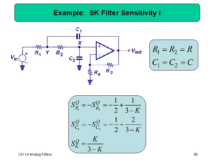
Example: SK Filter Sensitivity I CH 14 Analog Filters 80

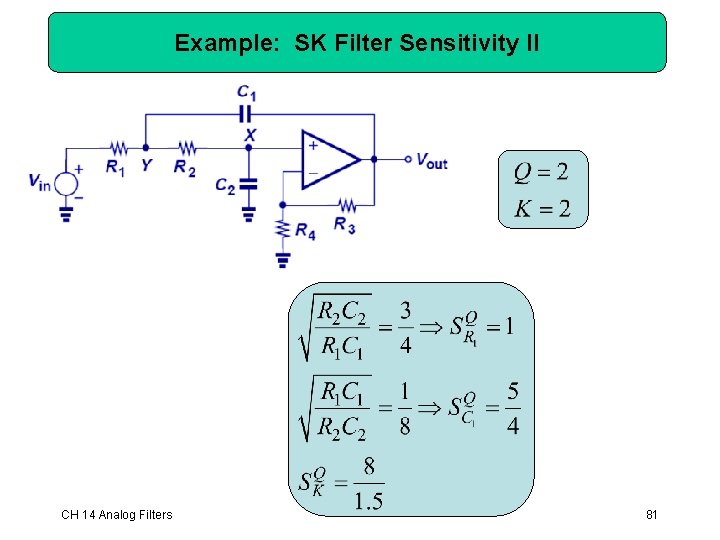
Example: SK Filter Sensitivity II CH 14 Analog Filters 81

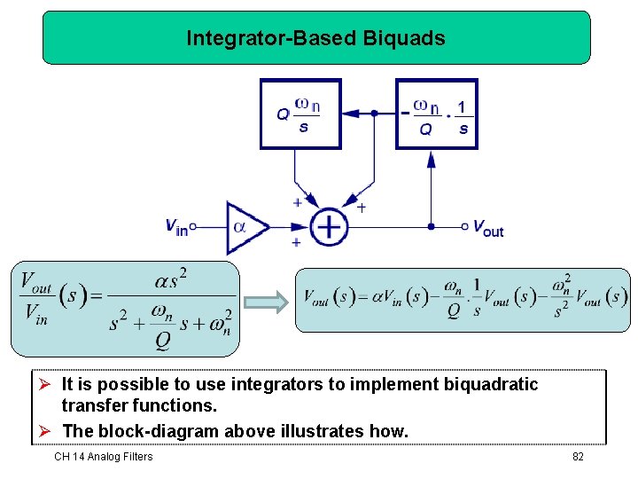
Integrator-Based Biquads Ø It is possible to use integrators to implement biquadratic transfer functions. Ø The block-diagram above illustrates how. CH 14 Analog Filters 82

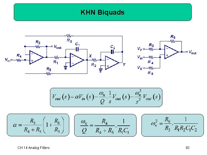
KHN Biquads CH 14 Analog Filters 83

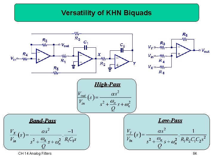
Versatility of KHN Biquads High-Pass Band-Pass CH 14 Analog Filters Low-Pass 84

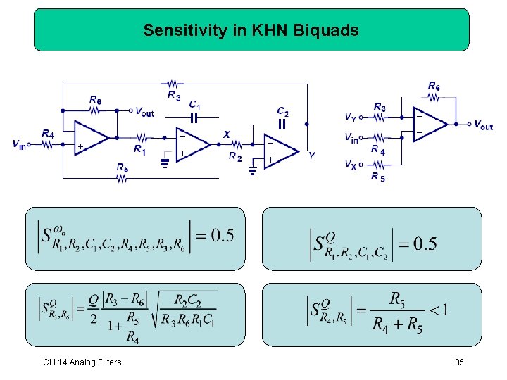
Sensitivity in KHN Biquads CH 14 Analog Filters 85

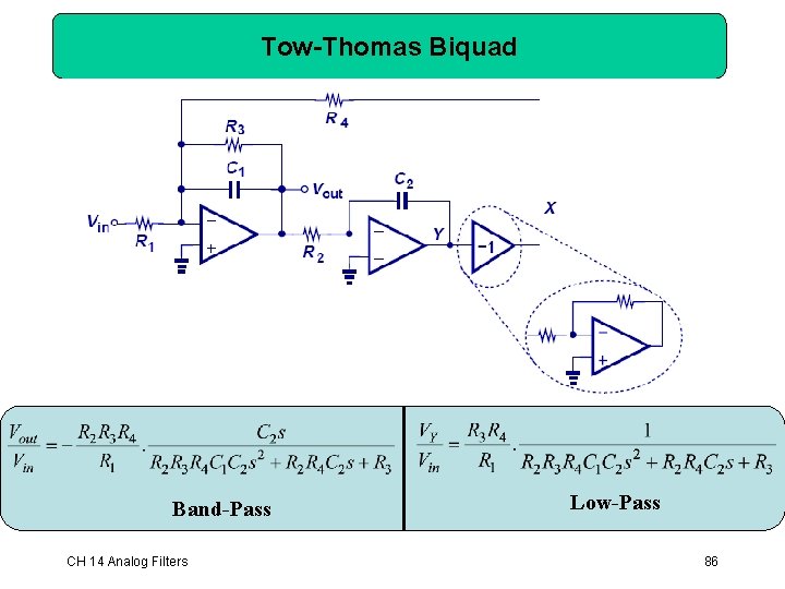
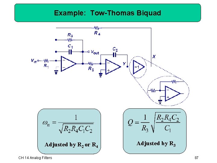
Tow-Thomas Biquad Band-Pass CH 14 Analog Filters Low-Pass 86

Example: Tow-Thomas Biquad Adjusted by R 2 or R 4 CH 14 Analog Filters Adjusted by R 3 87

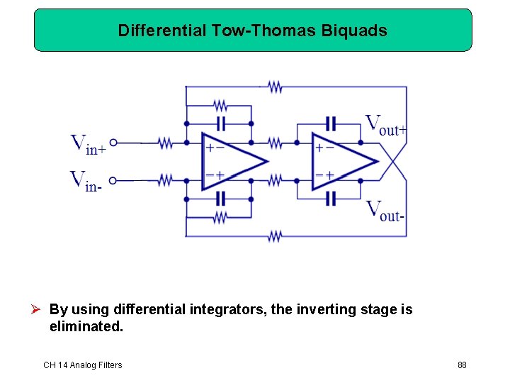
Differential Tow-Thomas Biquads Ø By using differential integrators, the inverting stage is eliminated. CH 14 Analog Filters 88

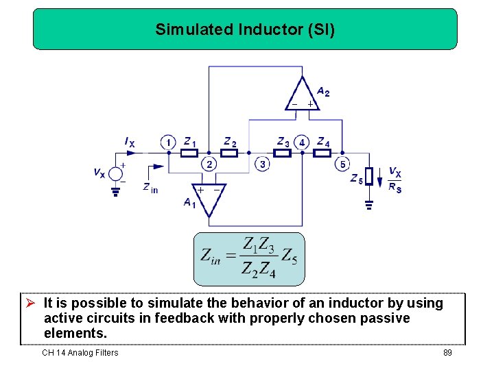
Simulated Inductor (SI) Ø It is possible to simulate the behavior of an inductor by using active circuits in feedback with properly chosen passive elements. CH 14 Analog Filters 89

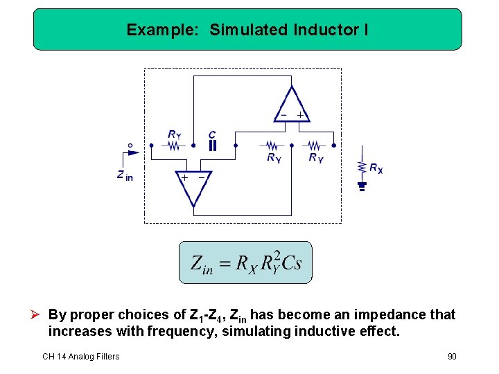
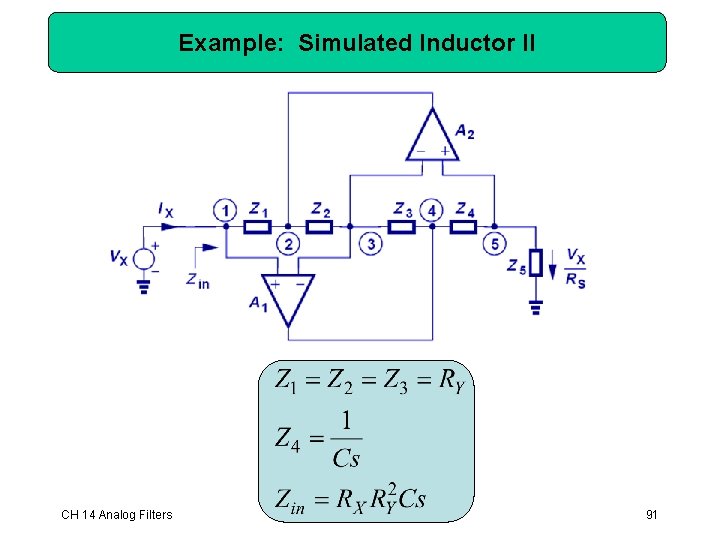
Example: Simulated Inductor I Ø By proper choices of Z 1 -Z 4, Zin has become an impedance that increases with frequency, simulating inductive effect. CH 14 Analog Filters 90

Example: Simulated Inductor II CH 14 Analog Filters 91

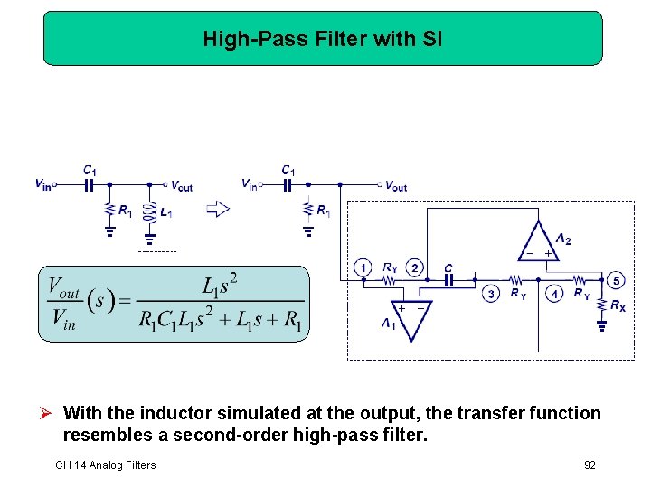
High-Pass Filter with SI Ø With the inductor simulated at the output, the transfer function resembles a second-order high-pass filter. CH 14 Analog Filters 92

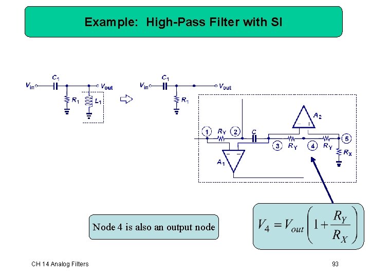
Example: High-Pass Filter with SI Node 4 is also an output node CH 14 Analog Filters 93

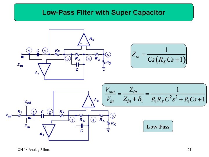
Low-Pass Filter with Super Capacitor Low-Pass CH 14 Analog Filters 94

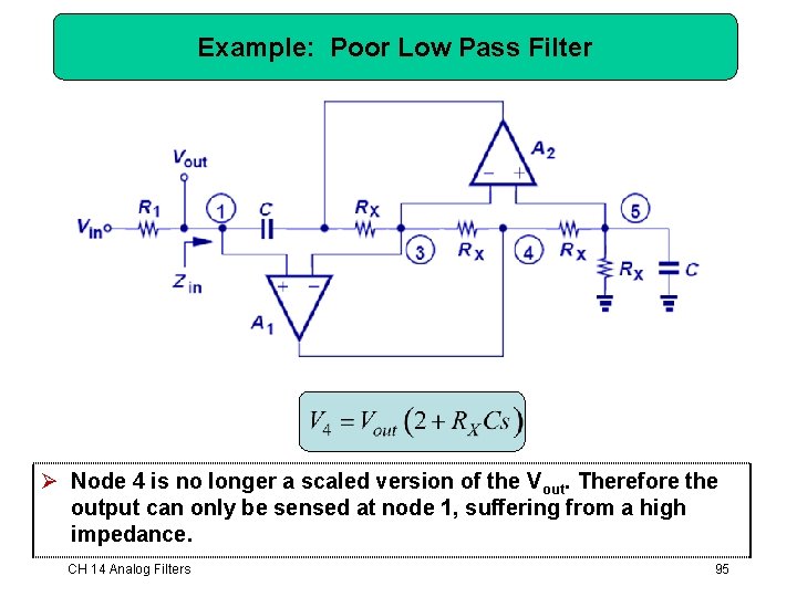
Example: Poor Low Pass Filter Ø Node 4 is no longer a scaled version of the Vout. Therefore the output can only be sensed at node 1, suffering from a high impedance. CH 14 Analog Filters 95

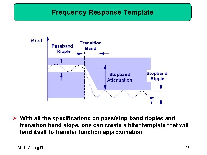
Frequency Response Template Ø With all the specifications on pass/stop band ripples and transition band slope, one can create a filter template that will lend itself to transfer function approximation. CH 14 Analog Filters 96

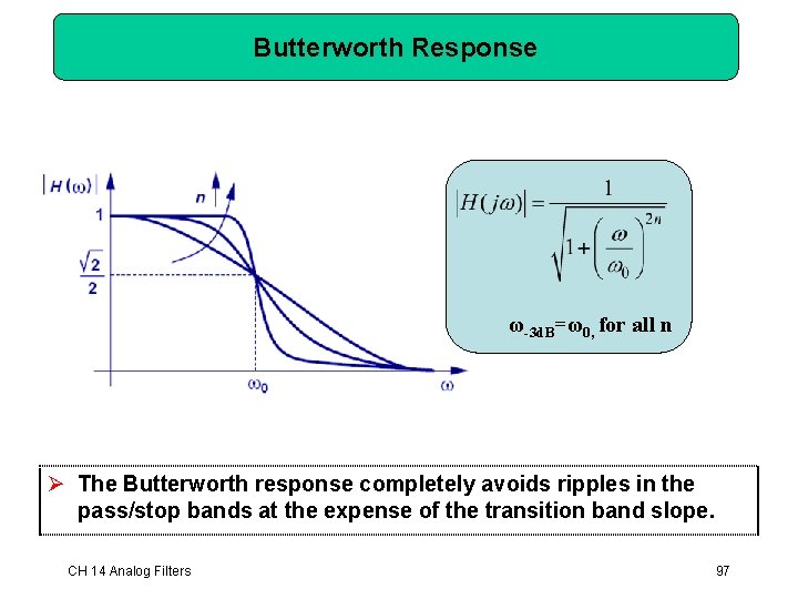
Butterworth Response ω-3 d. B=ω0, for all n Ø The Butterworth response completely avoids ripples in the pass/stop bands at the expense of the transition band slope. CH 14 Analog Filters 97

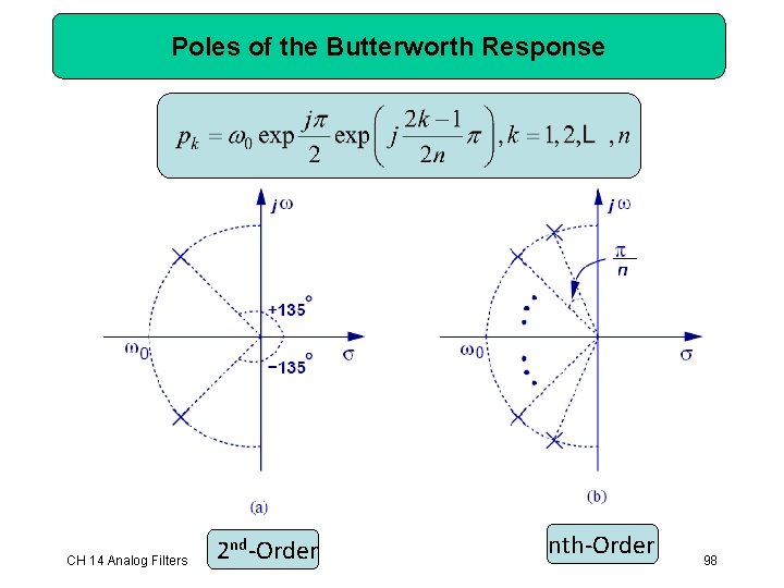
Poles of the Butterworth Response CH 14 Analog Filters 2 nd-Order nth-Order 98

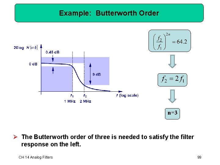
Example: Butterworth Order n=3 Ø The Butterworth order of three is needed to satisfy the filter response on the left. CH 14 Analog Filters 99

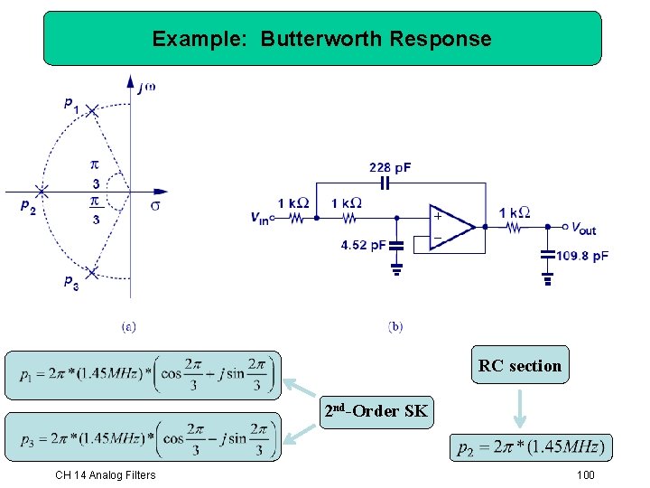
Example: Butterworth Response RC section 2 nd-Order SK CH 14 Analog Filters 100

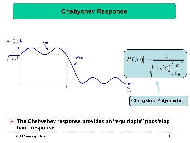
Chebyshev Response Chebyshev Polynomial Ø The Chebyshev response provides an “equiripple” pass/stop band response. CH 14 Analog Filters 101

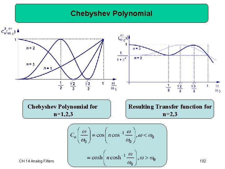
Chebyshev Polynomial for n=1, 2, 3 CH 14 Analog Filters Resulting Transfer function for n=2, 3 102

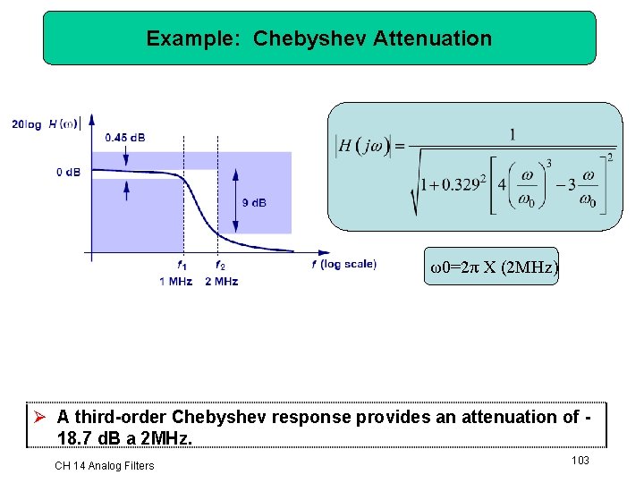
Example: Chebyshev Attenuation ω0=2π X (2 MHz) Ø A third-order Chebyshev response provides an attenuation of 18. 7 d. B a 2 MHz. CH 14 Analog Filters 103

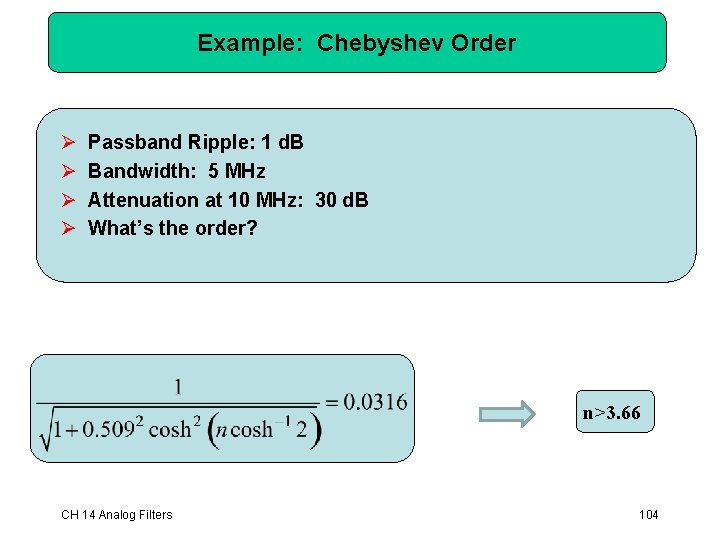
Example: Chebyshev Order Ø Ø Passband Ripple: 1 d. B Bandwidth: 5 MHz Attenuation at 10 MHz: 30 d. B What’s the order? n>3. 66 CH 14 Analog Filters 104

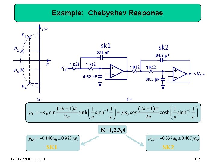
Example: Chebyshev Response K=1, 2, 3, 4 SK 1 CH 14 Analog Filters SK 2 105

Chapter 15 Digital CMOS Circuits Ø 15. 1 General Considerations Ø 15. 2 CMOS Inverter Ø 15. 3 CMOS NOR and NAND Gates 106

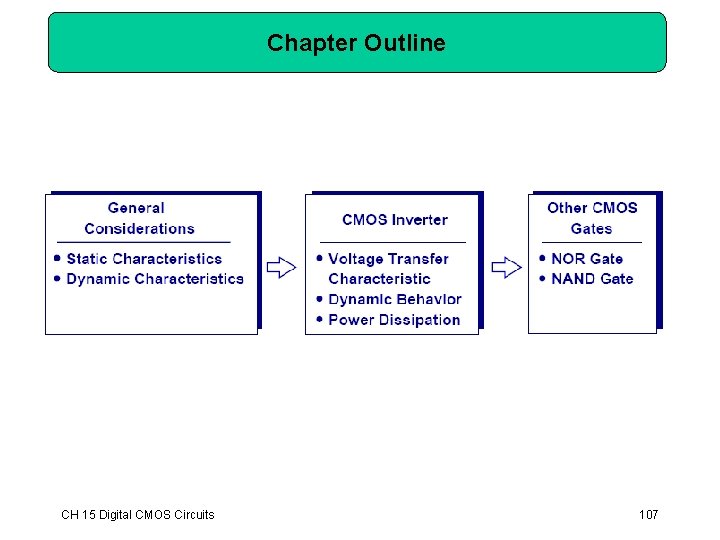
Chapter Outline CH 15 Digital CMOS Circuits 107

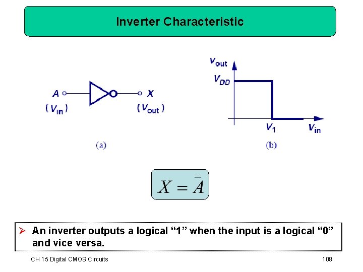
Inverter Characteristic Ø An inverter outputs a logical “ 1” when the input is a logical “ 0” and vice versa. CH 15 Digital CMOS Circuits 108

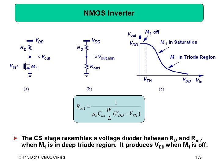
NMOS Inverter Ø The CS stage resembles a voltage divider between RD and Ron 1 when M 1 is in deep triode region. It produces VDD when M 1 is off. CH 15 Digital CMOS Circuits 109

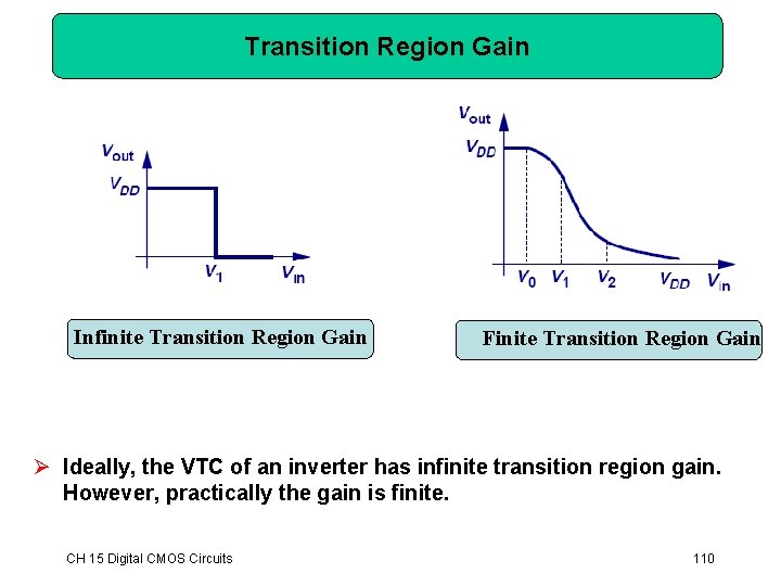
Transition Region Gain Infinite Transition Region Gain Finite Transition Region Gain Ø Ideally, the VTC of an inverter has infinite transition region gain. However, practically the gain is finite. CH 15 Digital CMOS Circuits 110

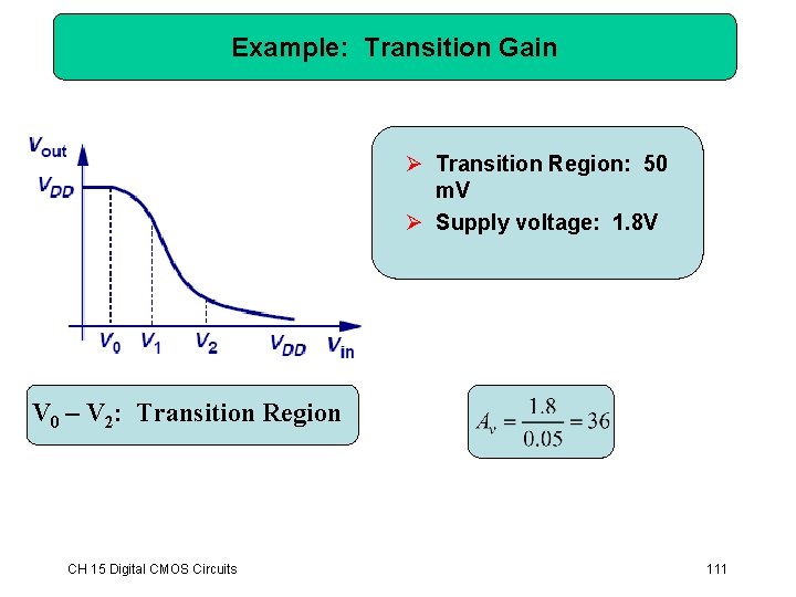
Example: Transition Gain Ø Transition Region: 50 m. V Ø Supply voltage: 1. 8 V V 0 – V 2: Transition Region CH 15 Digital CMOS Circuits 111

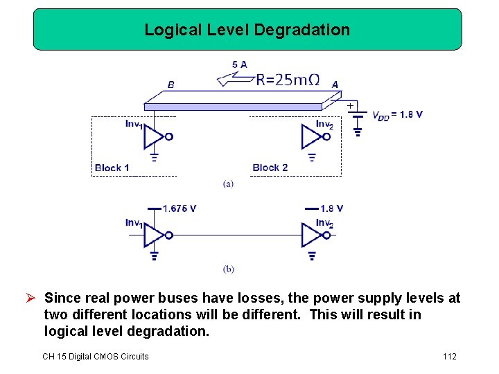
Logical Level Degradation Ø Since real power buses have losses, the power supply levels at two different locations will be different. This will result in logical level degradation. CH 15 Digital CMOS Circuits 112

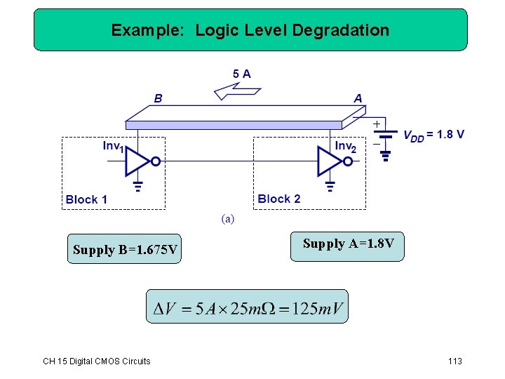
Example: Logic Level Degradation Supply B=1. 675 V CH 15 Digital CMOS Circuits Supply A=1. 8 V 113

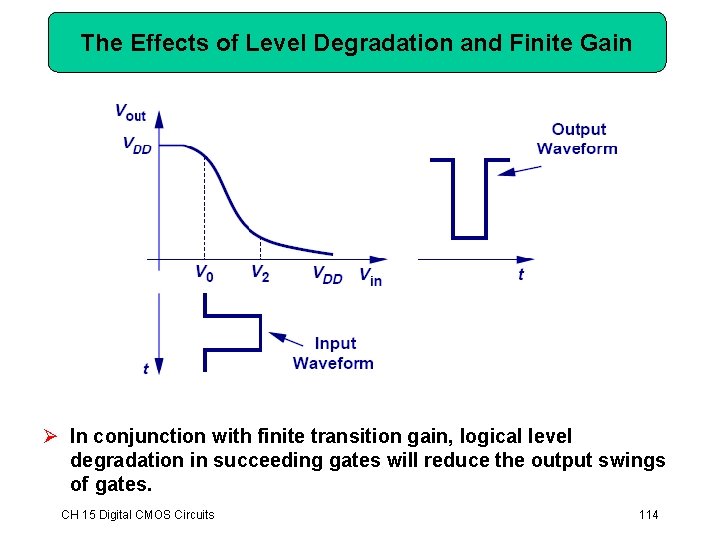
The Effects of Level Degradation and Finite Gain Ø In conjunction with finite transition gain, logical level degradation in succeeding gates will reduce the output swings of gates. CH 15 Digital CMOS Circuits 114

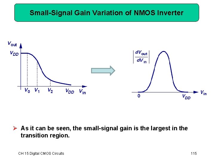
Small-Signal Gain Variation of NMOS Inverter Ø As it can be seen, the small-signal gain is the largest in the transition region. CH 15 Digital CMOS Circuits 115

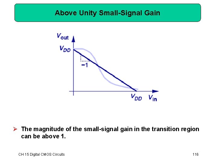
Above Unity Small-Signal Gain Ø The magnitude of the small-signal gain in the transition region can be above 1. CH 15 Digital CMOS Circuits 116

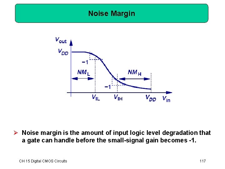
Noise Margin Ø Noise margin is the amount of input logic level degradation that a gate can handle before the small-signal gain becomes -1. CH 15 Digital CMOS Circuits 117

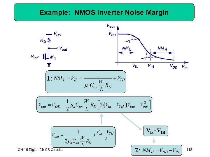
Example: NMOS Inverter Noise Margin 1: Vin=VIH CH 15 Digital CMOS Circuits 2: 118

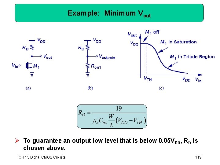
Example: Minimum Vout Ø To guarantee an output low level that is below 0. 05 VDD, RD is chosen above. CH 15 Digital CMOS Circuits 119

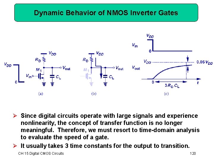
Dynamic Behavior of NMOS Inverter Gates Ø Since digital circuits operate with large signals and experience nonlinearity, the concept of transfer function is no longer meaningful. Therefore, we must resort to time-domain analysis to evaluate the speed of a gate. Ø It usually takes 3 time constants for the output to transition. CH 15 Digital CMOS Circuits 120

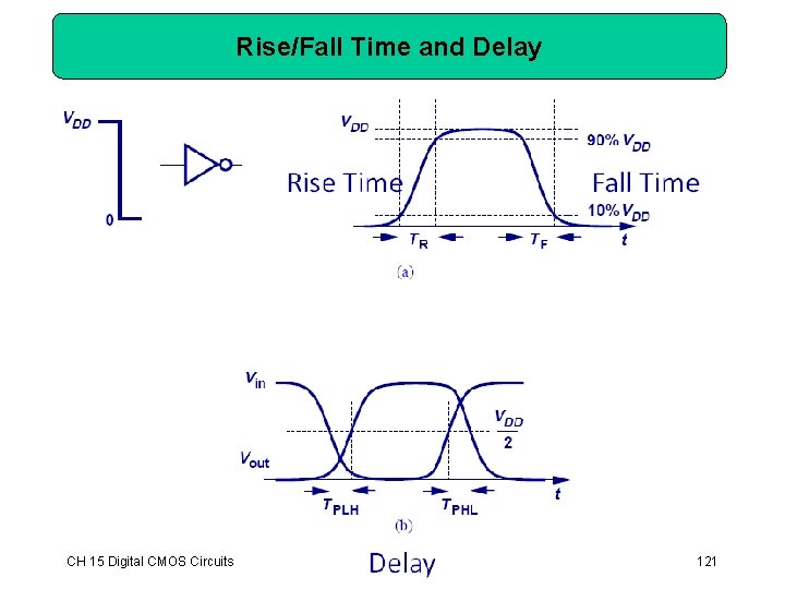
Rise/Fall Time and Delay CH 15 Digital CMOS Circuits 121

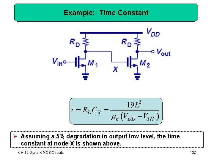
Example: Time Constant Ø Assuming a 5% degradation in output low level, the time constant at node X is shown above. CH 15 Digital CMOS Circuits 122

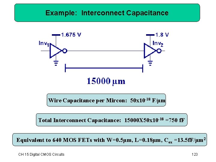
Example: Interconnect Capacitance Wire Capacitance per Mircon: 50 x 10 -18 F/µm Total Interconnect Capacitance: 15000 X 50 x 10 -18 =750 f. F Equivalent to 640 MOS FETs with W=0. 5µm, L=0. 18µm, Cox =13. 5 f. F/µm 2 CH 15 Digital CMOS Circuits 123

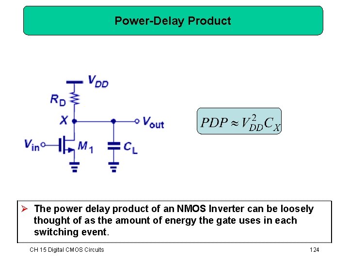
Power-Delay Product Ø The power delay product of an NMOS Inverter can be loosely thought of as the amount of energy the gate uses in each switching event. CH 15 Digital CMOS Circuits 124

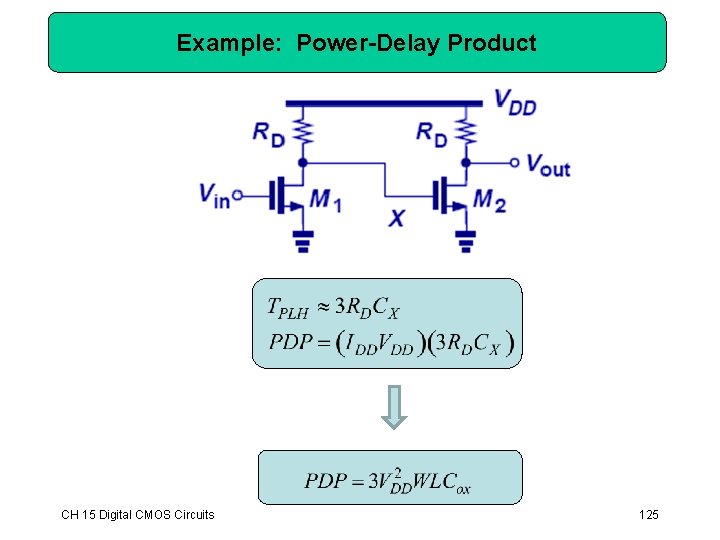
Example: Power-Delay Product CH 15 Digital CMOS Circuits 125

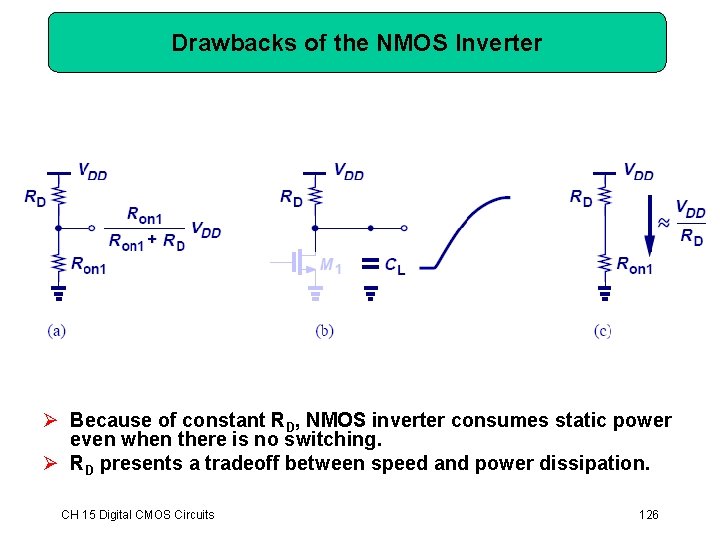
Drawbacks of the NMOS Inverter Ø Because of constant RD, NMOS inverter consumes static power even when there is no switching. Ø RD presents a tradeoff between speed and power dissipation. CH 15 Digital CMOS Circuits 126

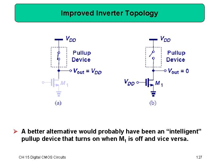
Improved Inverter Topology Ø A better alternative would probably have been an “intelligent” pullup device that turns on when M 1 is off and vice versa. CH 15 Digital CMOS Circuits 127

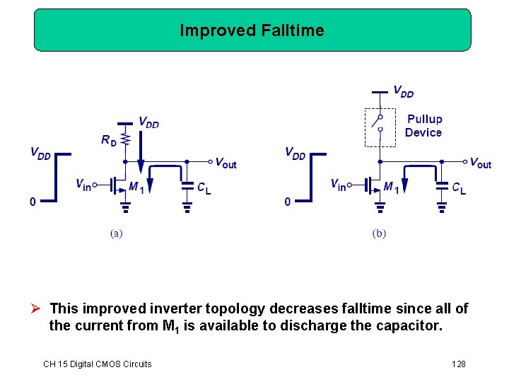
Improved Falltime Ø This improved inverter topology decreases falltime since all of the current from M 1 is available to discharge the capacitor. CH 15 Digital CMOS Circuits 128

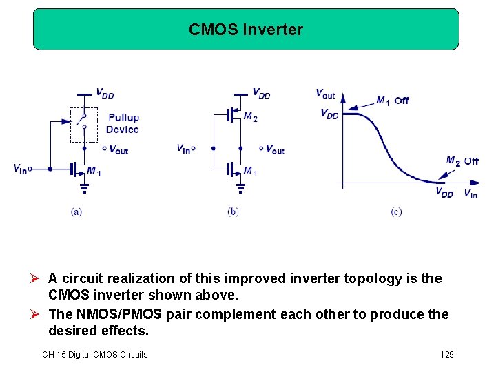
CMOS Inverter Ø A circuit realization of this improved inverter topology is the CMOS inverter shown above. Ø The NMOS/PMOS pair complement each other to produce the desired effects. CH 15 Digital CMOS Circuits 129

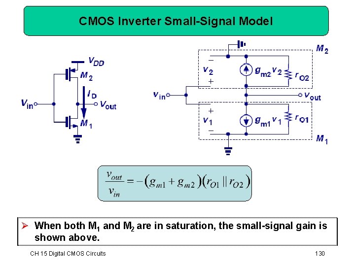
CMOS Inverter Small-Signal Model Ø When both M 1 and M 2 are in saturation, the small-signal gain is shown above. CH 15 Digital CMOS Circuits 130

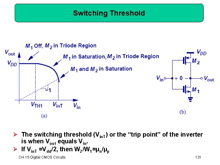
Switching Threshold Ø The switching threshold (Vin. T) or the “trip point” of the inverter is when Vout equals Vin. Ø If Vin. T =Vdd/2, then W 2/W 1=µn/µp CH 15 Digital CMOS Circuits 131

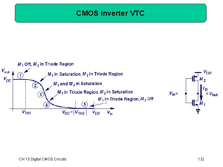
CMOS Inverter VTC CH 15 Digital CMOS Circuits 132

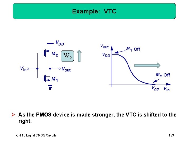
Example: VTC W 2 Ø As the PMOS device is made stronger, the VTC is shifted to the right. CH 15 Digital CMOS Circuits 133

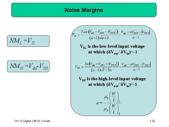
Noise Margins NML =VIL is the low-level input voltage at which (δVout/ δVin)=-1 NMH =Vdd-VIH is the high-level input voltage at which (δVout/ δVin)=-1 CH 15 Digital CMOS Circuits 134

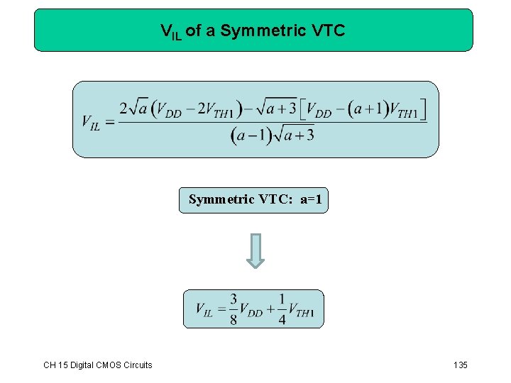
VIL of a Symmetric VTC: a=1 CH 15 Digital CMOS Circuits 135

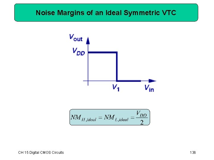
Noise Margins of an Ideal Symmetric VTC CH 15 Digital CMOS Circuits 136

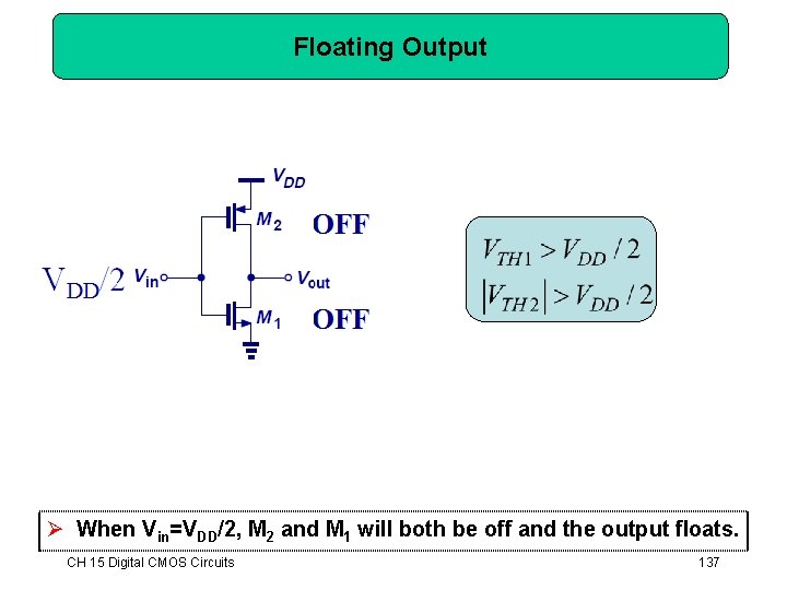
Floating Output Ø When Vin=VDD/2, M 2 and M 1 will both be off and the output floats. CH 15 Digital CMOS Circuits 137

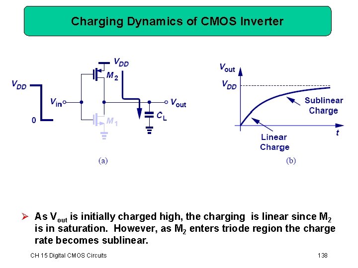
Charging Dynamics of CMOS Inverter Ø As Vout is initially charged high, the charging is linear since M 2 is in saturation. However, as M 2 enters triode region the charge rate becomes sublinear. CH 15 Digital CMOS Circuits 138

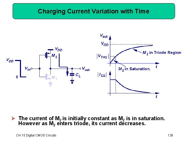
Charging Current Variation with Time Ø The current of M 2 is initially constant as M 2 is in saturation. However as M 2 enters triode, its current decreases. CH 15 Digital CMOS Circuits 139

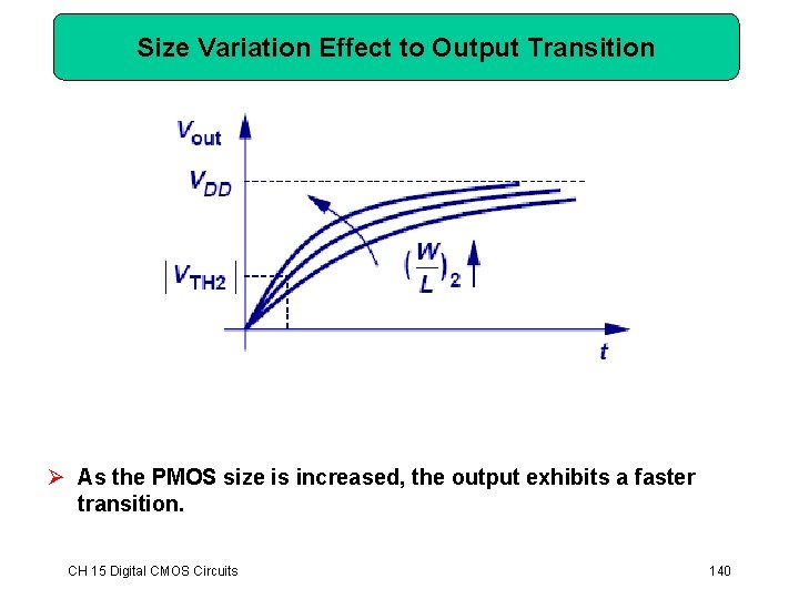
Size Variation Effect to Output Transition Ø As the PMOS size is increased, the output exhibits a faster transition. CH 15 Digital CMOS Circuits 140

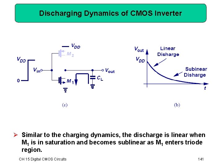
Discharging Dynamics of CMOS Inverter Ø Similar to the charging dynamics, the discharge is linear when M 1 is in saturation and becomes sublinear as M 1 enters triode region. CH 15 Digital CMOS Circuits 141

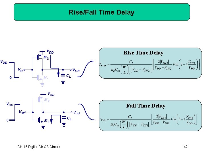
Rise/Fall Time Delay Rise Time Delay Fall Time Delay CH 15 Digital CMOS Circuits 142

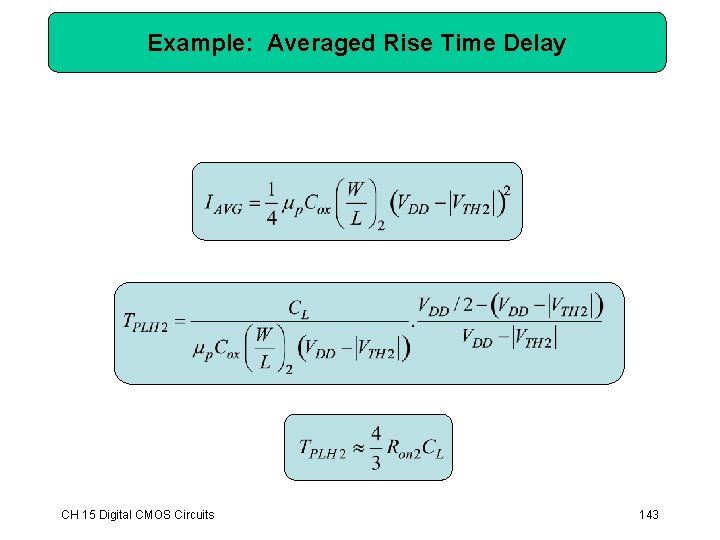
Example: Averaged Rise Time Delay CH 15 Digital CMOS Circuits 143

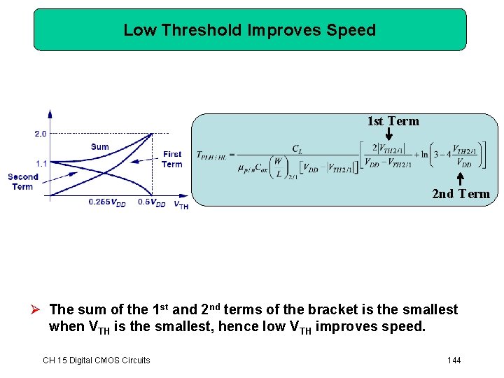
Low Threshold Improves Speed 1 st Term 2 nd Term Ø The sum of the 1 st and 2 nd terms of the bracket is the smallest when VTH is the smallest, hence low VTH improves speed. CH 15 Digital CMOS Circuits 144

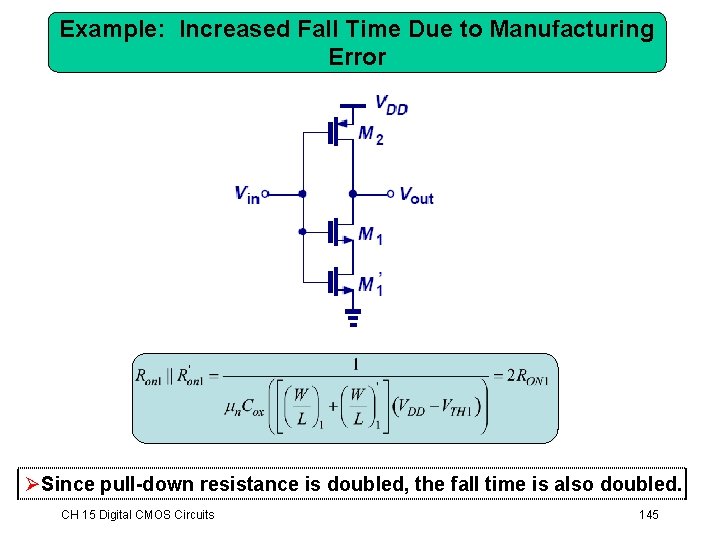
Example: Increased Fall Time Due to Manufacturing Error ØSince pull-down resistance is doubled, the fall time is also doubled. CH 15 Digital CMOS Circuits 145

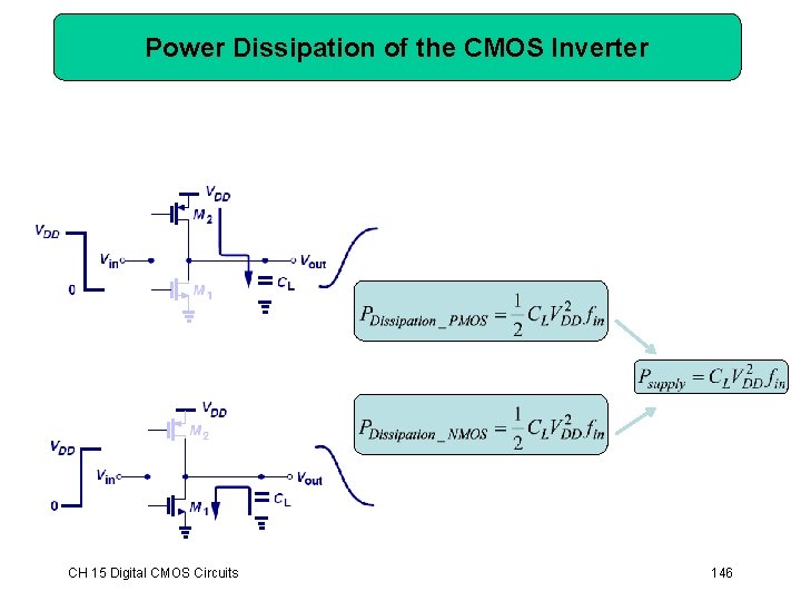
Power Dissipation of the CMOS Inverter CH 15 Digital CMOS Circuits 146

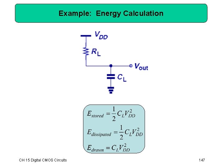
Example: Energy Calculation CH 15 Digital CMOS Circuits 147

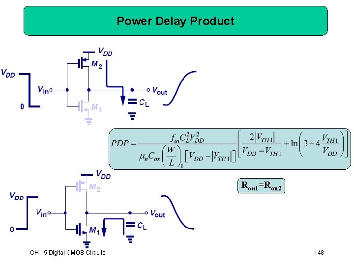
Power Delay Product Ron 1=Ron 2 CH 15 Digital CMOS Circuits 148

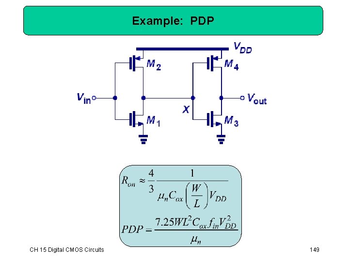
Example: PDP CH 15 Digital CMOS Circuits 149

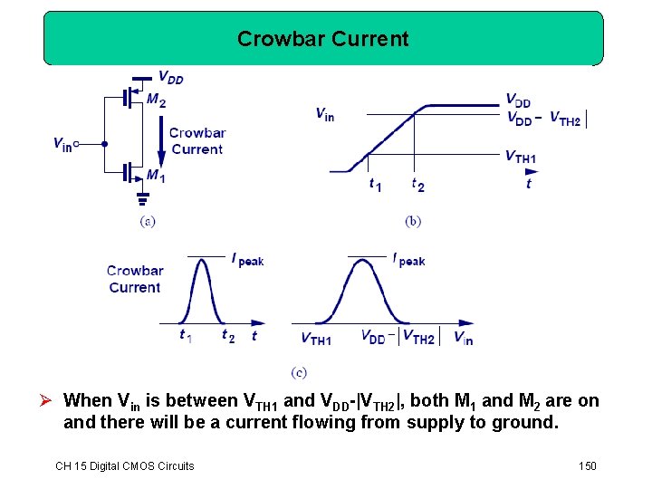
Crowbar Current Ø When Vin is between VTH 1 and VDD-|VTH 2|, both M 1 and M 2 are on and there will be a current flowing from supply to ground. CH 15 Digital CMOS Circuits 150

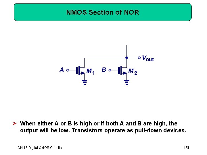
NMOS Section of NOR Ø When either A or B is high or if both A and B are high, the output will be low. Transistors operate as pull-down devices. CH 15 Digital CMOS Circuits 151

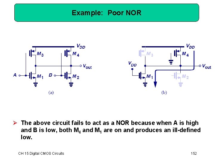
Example: Poor NOR Ø The above circuit fails to act as a NOR because when A is high and B is low, both M 4 and M 1 are on and produces an ill-defined low. CH 15 Digital CMOS Circuits 152

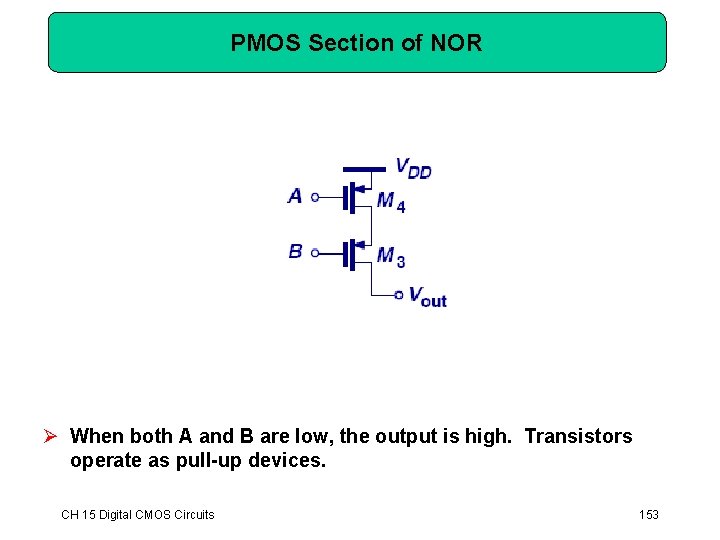
PMOS Section of NOR Ø When both A and B are low, the output is high. Transistors operate as pull-up devices. CH 15 Digital CMOS Circuits 153

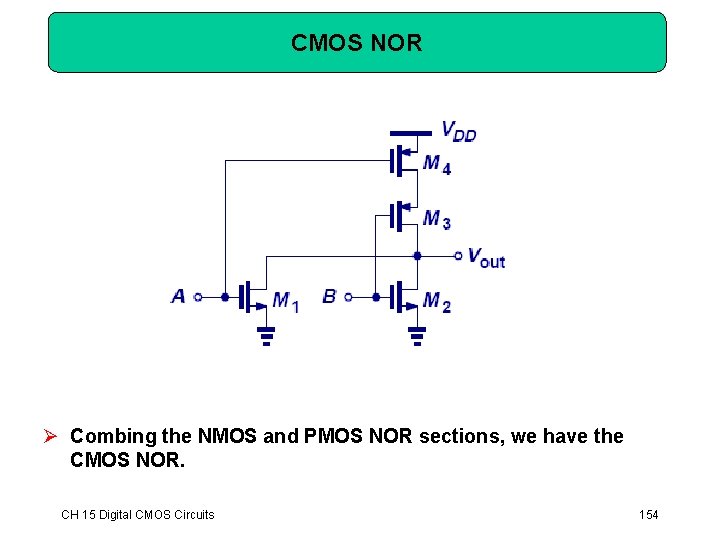
CMOS NOR Ø Combing the NMOS and PMOS NOR sections, we have the CMOS NOR. CH 15 Digital CMOS Circuits 154

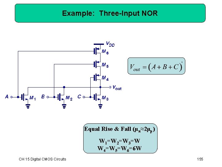
Example: Three-Input NOR Equal Rise & Fall (µn≈2µp) W 1=W 2=W 3=W W 4=W 5=W 6=6 W CH 15 Digital CMOS Circuits 155

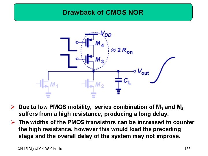
Drawback of CMOS NOR Ø Due to low PMOS mobility, series combination of M 3 and M 4 suffers from a high resistance, producing a long delay. Ø The widths of the PMOS transistors can be increased to counter the high resistance, however this would load the preceding stage and the overall delay of the system may not improve. CH 15 Digital CMOS Circuits 156

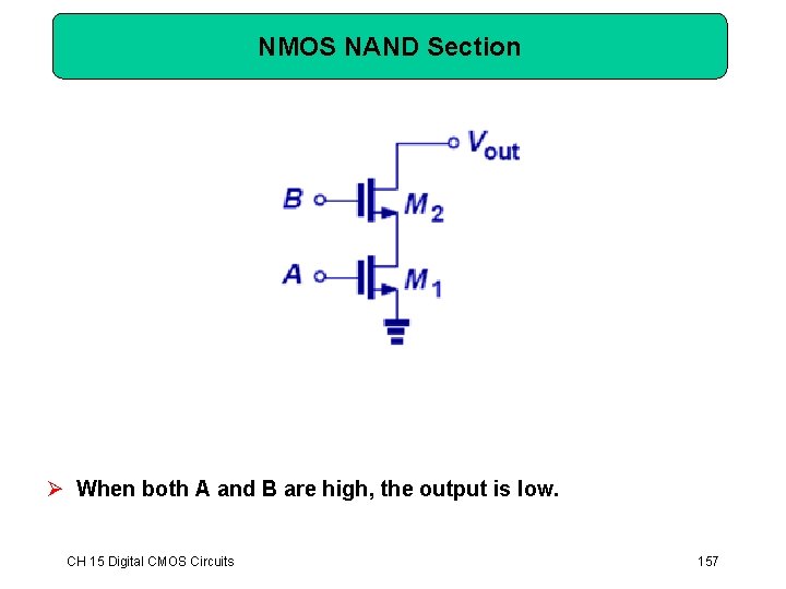
NMOS NAND Section Ø When both A and B are high, the output is low. CH 15 Digital CMOS Circuits 157

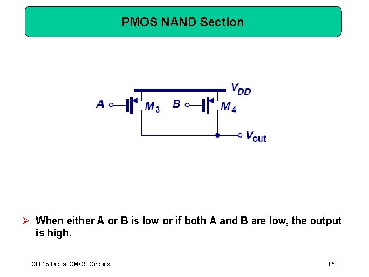
PMOS NAND Section Ø When either A or B is low or if both A and B are low, the output is high. CH 15 Digital CMOS Circuits 158

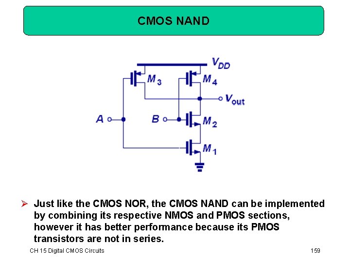
CMOS NAND Ø Just like the CMOS NOR, the CMOS NAND can be implemented by combining its respective NMOS and PMOS sections, however it has better performance because its PMOS transistors are not in series. CH 15 Digital CMOS Circuits 159

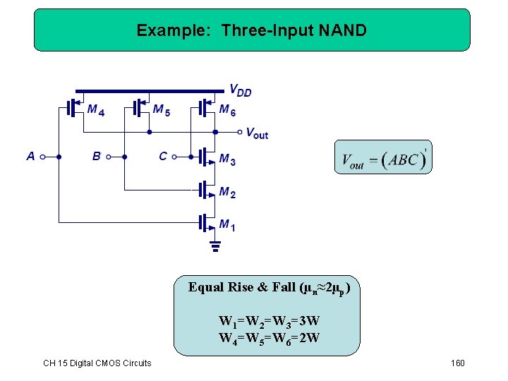
Example: Three-Input NAND Equal Rise & Fall (µn≈2µp) W 1=W 2=W 3=3 W W 4=W 5=W 6=2 W CH 15 Digital CMOS Circuits 160

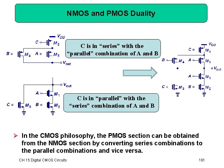
NMOS and PMOS Duality C is in “series” with the “parallel” combination of A and B C is in “parallel” with the “series” combination of A and B Ø In the CMOS philosophy, the PMOS section can be obtained from the NMOS section by converting series combinations to the parallel combinations and vice versa. CH 15 Digital CMOS Circuits 161