The Examination of Residuals Examination of Residuals The

The Examination of Residuals

Examination of Residuals The fitting of models to data is done using an iterative approach. The first step is to fit a simple model (usually a linear model). The next step is examine the validity of the model. This is usually achieved by examination of residuals. If the model proves to be incorrect, the residuals will also point to improvements in the model.

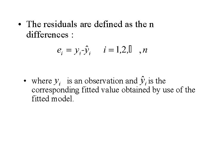
• The residuals are defined as the n differences : • where is an observation and is the corresponding fitted value obtained by use of the fitted model.

• Many of the statistical procedures used in linear and nonlinear regression analysis are based certain assumptions about the random departures from the proposed model. • Namely; the random departures are assumed i) to have zero mean, ii) to have a constant variance, s 2, iii) independent, and iv) follow a normal distribution.

Thus if the fitted model is correct, • the residuals should exhibit tendencies that tend to confirm the above assumptions, or at least, should not exhibit a denial of the assumptions.

The Examination of Residuals

• The residuals are defined as the n differences : • where is an observation and is the corresponding fitted value obtained by use of the fitted model.

• Many of the statistical procedures used in linear and nonlinear regression analysis are based certain assumptions about the random departures from the proposed model. • Namely; the random departures are assumed i) to have zero mean, ii) to have a constant variance, s 2, iii) independent, and iv) follow a normal distribution. Thus if the fitted model is correct, • the residuals should exhibit tendencies that tend to confirm the above assumptions, or at least, should not exhibit a denial of the assumptions.

The principal ways of plotting the residuals ei are: 1. Overall. 2. In time sequence, if the order is known. 3. Against the fitted values 4. Against the independent variables xij for each value of j In addition to these basic plots, the residuals should also be plotted 5. In any way that is sensible for the particular problem under consideration,

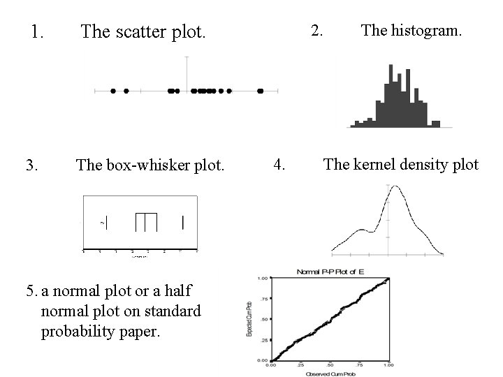
Overall Plot The residuals can be plotted in an overall plot in several ways.

1. The scatter plot. 3. The box-whisker plot. 5. a normal plot or a half normal plot on standard probability paper. 2. 4. The histogram. The kernel density plot

• The standard statistical test for testing Normality are: 1. The Kolmogorov-Smirnov test. 2. The Chi-square goodness of fit test

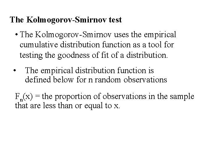
The Kolmogorov-Smirnov test • The Kolmogorov-Smirnov uses the empirical cumulative distribution function as a tool for testing the goodness of fit of a distribution. • The empirical distribution function is defined below for n random observations Fn(x) = the proportion of observations in the sample that are less than or equal to x.

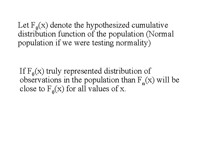
Let F 0(x) denote the hypothesized cumulative distribution function of the population (Normal population if we were testing normality) If F 0(x) truly represented distribution of observations in the population than Fn(x) will be close to F 0(x) for all values of x.

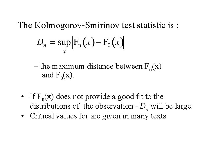
The Kolmogorov-Smirinov test statistic is : = the maximum distance between Fn(x) and F 0(x). • If F 0(x) does not provide a good fit to the distributions of the observation - Dn will be large. • Critical values for are given in many texts

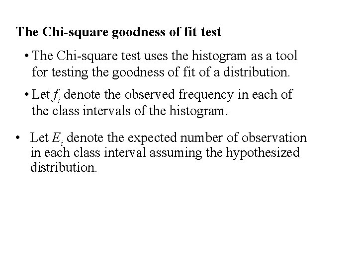
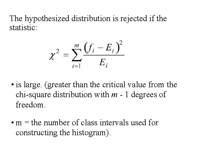
The Chi-square goodness of fit test • The Chi-square test uses the histogram as a tool for testing the goodness of fit of a distribution. • Let fi denote the observed frequency in each of the class intervals of the histogram. • Let Ei denote the expected number of observation in each class interval assuming the hypothesized distribution.

The hypothesized distribution is rejected if the statistic: • is large. (greater than the critical value from the chi-square distribution with m - 1 degrees of freedom. • m = the number of class intervals used for constructing the histogram).

Note. The in the above tests it is assumed that the residuals are independent with a common variance of s 2. This is not completely accurate for this reason: Although theoretical random errors ei are all assumed to be independent with the same variance s 2, the residuals are not independent and they also do not have the same variance.

They will however be approximately independent with common variance if the sample size is large relative to the number of parameters in the model. It is important to keep this in mind when judging residuals when the number of observations is close to the number of parameters in the model.

Time Sequence Plot The residuals should exhibit a pattern of independence. If the data was collected in time there could be a strong possibility that the random departures from the model are autocorrelated.

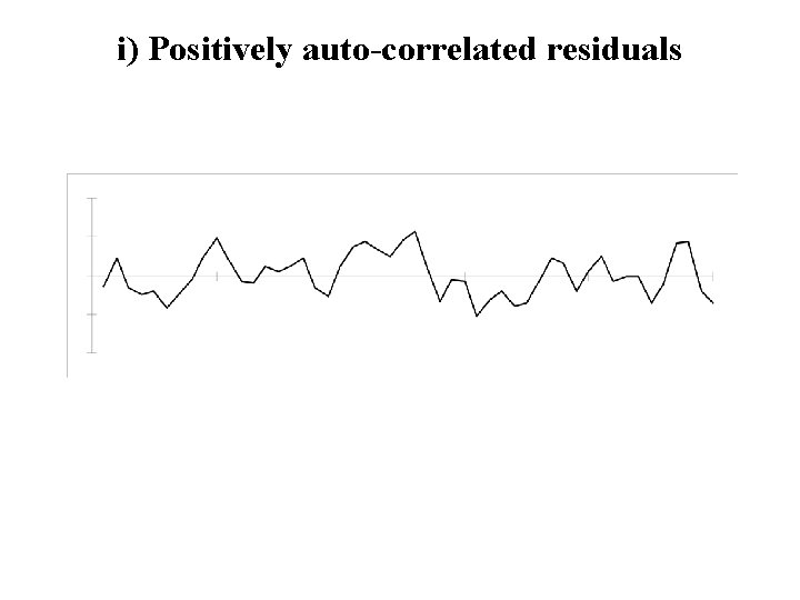
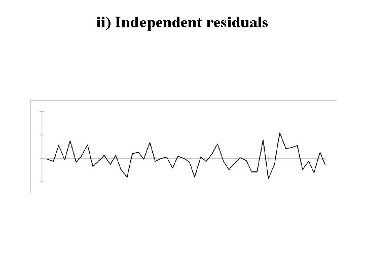
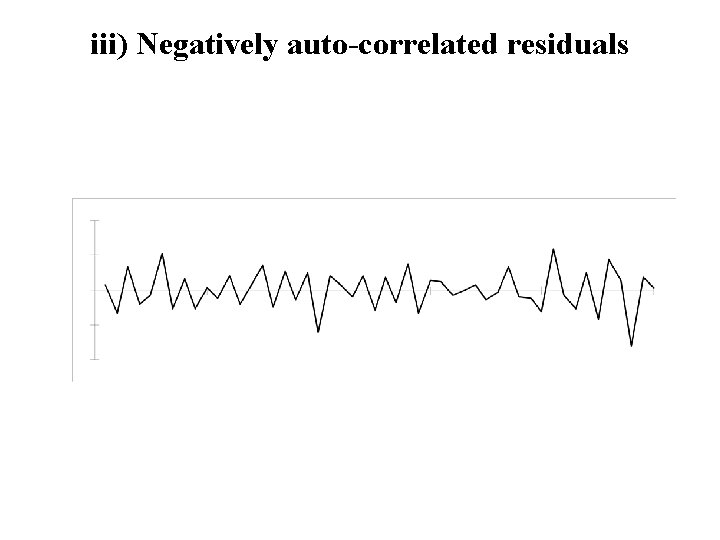
Namely the random departures for observations that were taken at neighbouring points in time are autocorrelated. This autocorrelation can sometimes be seen in a time sequence plot. The following three graphs show a sequence of residuals that are respectively i) positively autocorrelated , ii) independent and iii) negatively autocorrelated.

i) Positively auto-correlated residuals

ii) Independent residuals

iii) Negatively auto-correlated residuals

There are several statistics and statistical tests that can also pick out autocorrelation amongst the residuals. The most common are: i) iii) The Durbin Watson statistic The autocorrelation function The runs test

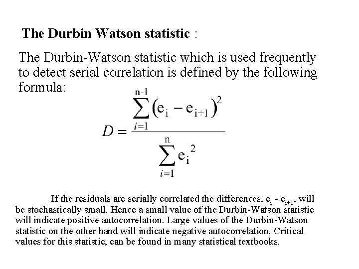
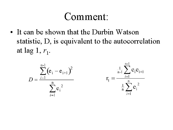
The Durbin Watson statistic : The Durbin-Watson statistic which is used frequently to detect serial correlation is defined by the following formula: If the residuals are serially correlated the differences, ei - ei+1, will be stochastically small. Hence a small value of the Durbin-Watson statistic will indicate positive autocorrelation. Large values of the Durbin-Watson statistic on the other hand will indicate negative autocorrelation. Critical values for this statistic, can be found in many statistical textbooks.

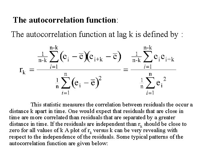
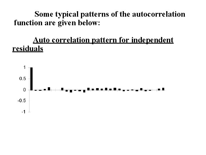
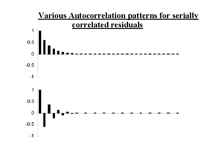
The autocorrelation function: The autocorrelation function at lag k is defined by : This statistic measures the correlation between residuals the occur a distance k apart in time. One would expect that residuals that are close in time are more correlated than residuals that are separated by a greater distance in time. If the residuals are independent than rk should be close to zero for all values of k A plot of rk versus k can be very revealing with respect to the independence of the residuals. Some typical patterns of the autocorrelation function are given below:

This statistic measures the correlation between residuals the occur a distance k apart in time. One would expect that residuals that are close in time are more correlated than residuals that are separated by a greater distance in time. If the residuals are independent than rk should be close to zero for all values of k A plot of rk versus k can be very revealing with respect to the independence of the residuals.

Some typical patterns of the autocorrelation function are given below: Auto correlation pattern for independent residuals

Various Autocorrelation patterns for serially correlated residuals

Comment: • It can be shown that the Durbin Watson statistic, D, is equivalent to the autocorrelation at lag 1, r 1.

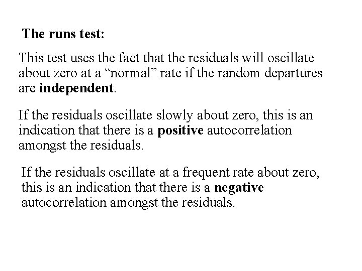
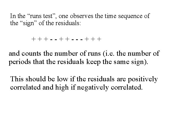
The runs test: This test uses the fact that the residuals will oscillate about zero at a “normal” rate if the random departures are independent. If the residuals oscillate slowly about zero, this is an indication that there is a positive autocorrelation amongst the residuals. If the residuals oscillate at a frequent rate about zero, this is an indication that there is a negative autocorrelation amongst the residuals.

In the “runs test”, one observes the time sequence of the “sign” of the residuals: +++---+++ and counts the number of runs (i. e. the number of periods that the residuals keep the same sign). This should be low if the residuals are positively correlated and high if negatively correlated.

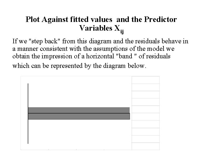
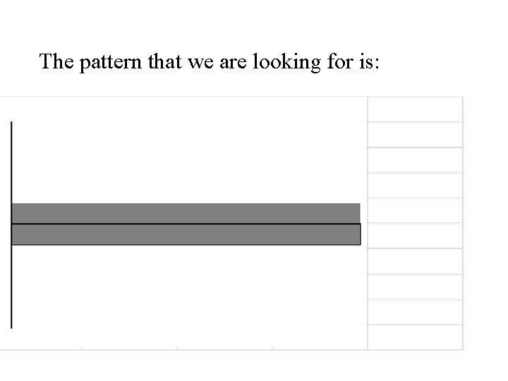
Plot Against fitted values and the Predictor Variables Xij If we "step back" from this diagram and the residuals behave in a manner consistent with the assumptions of the model we obtain the impression of a horizontal "band " of residuals which can be represented by the diagram below.

Individual observations lying considerably outside of this band indicate that the observation may be and outlier. An outlier is an observation that is not following the normal pattern of the other observations. Such an observation can have a considerable effect on the estimation of the parameters of a model. Sometimes the outlier has occurred because of a typographical error. If this is the case and it is detected than a correction can be made. If the outlier occurs for other (and more natural) reasons it may be appropriate to construct a model that incorporates the occurrence of outliers.

If our "step back" view of the residuals resembled any of those shown below we should conclude that assumptions about the model are incorrect. Each pattern may indicate that a different assumption may have to be made to explain the “abnormal” residual pattern. a) b)

Pattern a) indicates that the variance the random departures is not constant (homogeneous) but increases as the value along the horizontal axis increases (time, or one of the independent variables). This indicates that a weighted least squares analysis should be used. The second pattern, b) indicates that the mean value of the residuals is not zero. This is usually because the model (linear or non linear) has not been correctly specified. Linear and quadratic terms have been omitted that should have been included in the model.

Example – Analysis of Residuals Motor Vehicle Data Dependent = mpg Independent = Engine size, horsepower and weight

When a linear model was fit and residuals examined graphically the following plot resulted:

The pattern that we are looking for is:

The pattern that was found is: This indicates a nonlinear relationship: This can be handle by adding polynomial terms (quadratic, cubic, quartic etc. ) of the independent variables or transforming the dependent variable

Performing the log transformation on the dependent variable (mpg) results in the following residual plot There still remains some non linearity

The log transformation

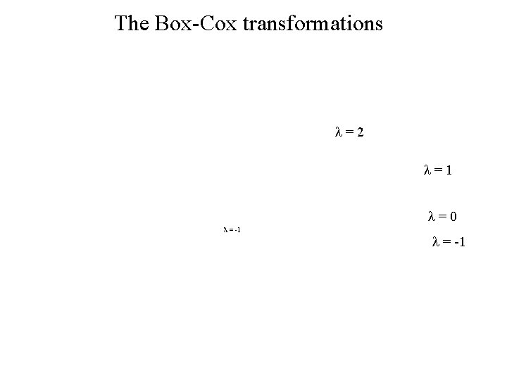
The Box-Cox transformations l=2 l=1 l=0 l = -1

The log (l = 0) transformation was not totally successful - try moving further down the staircase of the family of transformations (l = -0. 5)

try moving a bit further down the staircase of the family of transformations (l = -1. 0)

The results after deleting the outlier are given below:

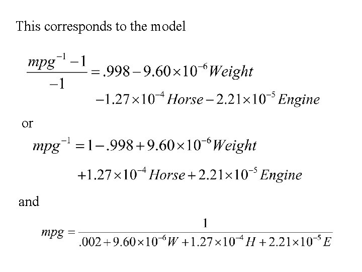
This corresponds to the model or and

Checking normality with a P-P plot