Chapter 5 Residuals Residual Plots Influential points Residuals

Residuals (error) • The vertical deviation between the observations & the LSRL • the

Residual plot • A scatterplot of the (x, residual) pairs. • Residuals can be

Range of Motion 35 154 24 142 40 137 31 133 28 122 25

Residuals x Residual plots are the same no matter if plotted against x or

Coefficient of determination • r 2 • gives the proportion of variation in y

Age Range of Motion 35 154 24 142 40 137 31 133 28 122

Age Range of Motion 35 154 SSy = 1564. 917 24 142 SSy =

Interpretation of 2 r Approximately r 2% of the variation in y can be

Computer-generated regression analysis of knee surgery Be sure to convert r 2 data: NEVER

Outlier – • In a regression setting, an outlier is a data point with

Influential point • A point that influences where the LSRL is located • If

Racket Resonance Acceleration (Hz) (m/sec) 1 105 36. 0 2 106 35. 0 3

(189, 30) could be influential. Remove & recalculate LSRL

(189, 30) was influential since it moved the LSRL

Which of these measures are resistant? • LSRL • Correlation coefficient • Coefficient of

Slides: 20

Download presentation

Chapter 5 Residuals, Residual Plots, & Influential points

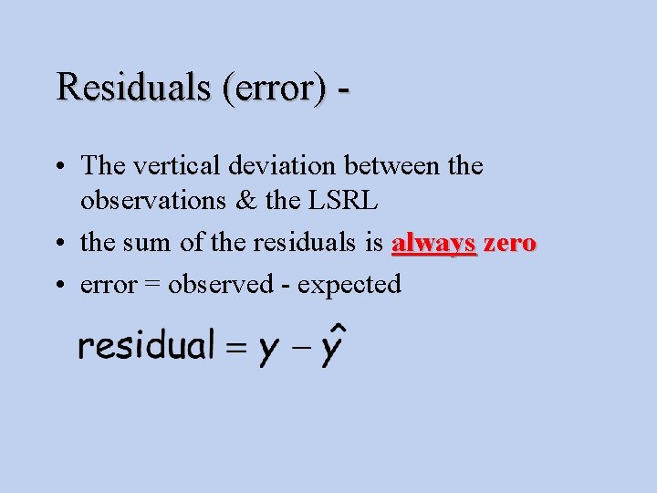
Residuals (error) • The vertical deviation between the observations & the LSRL • the sum of the residuals is always zero • error = observed - expected

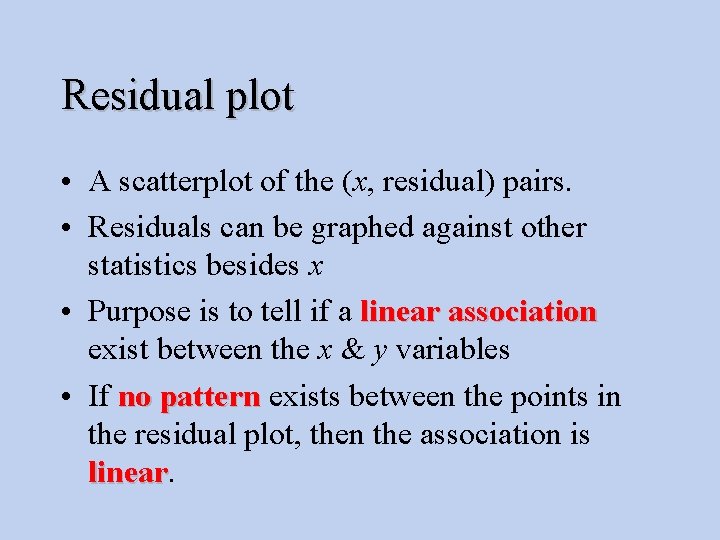
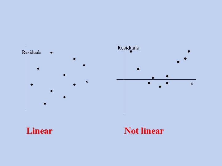
Residual plot • A scatterplot of the (x, residual) pairs. • Residuals can be graphed against other statistics besides x • Purpose is to tell if a linear association exist between the x & y variables • If no pattern exists between the points in the residual plot, then the association is linear

Linear Not linear

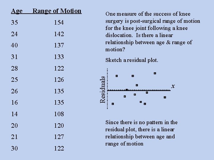
Range of Motion 35 154 24 142 40 137 31 133 28 122 25 126 26 135 14 108 20 120 21 127 30 122 One measure of the success of knee surgery is post-surgical range of motion for the knee joint following a knee dislocation. Is there a linear relationship between age & range of motion? Sketch a residual plot. Residuals Age x Since there is no pattern in the residual plot, there is a linear relationship between age and range of motion

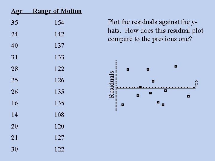
Range of Motion 35 154 24 142 40 137 31 133 28 122 25 126 26 135 14 108 20 120 21 127 30 122 Plot the residuals against the yhats. How does this residual plot compare to the previous one? Residuals Age

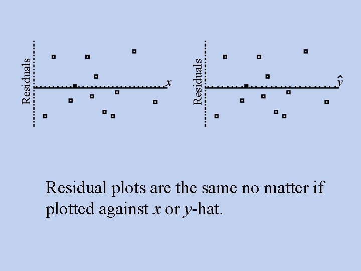
Residuals x Residual plots are the same no matter if plotted against x or y-hat.

Coefficient of determination • r 2 • gives the proportion of variation in y that can be attributed to an approximate linear relationship between x & y • remains the same no matter which variable is labeled x

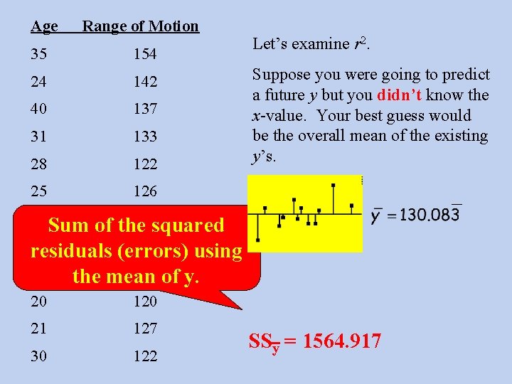
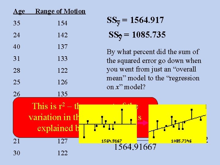
Age Range of Motion 35 154 24 142 40 137 31 133 28 122 25 126 Let’s examine r 2. Suppose you were going to predict a future y but you didn’t know the x-value. Your best guess would be the overall mean of the existing y’s. 26 135 Sum of the squared 16 135 residuals (errors) using 14 108 of y. the mean 20 120 21 127 30 122 SSy = 1564. 917

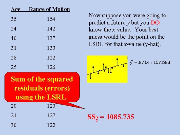
Age Range of Motion 35 154 24 142 40 137 31 133 28 122 25 126 Now suppose you were going to predict a future y but you DO know the x-value. Your best guess would be the point on the LSRL for that x-value (y-hat). 26 Sum of the 135 squared 16 residuals (errors) 135 14 using the LSRL. 108 20 120 21 127 30 122 SSy = 1085. 735

Age Range of Motion 35 154 SSy = 1564. 917 24 142 SSy = 1085. 735 40 137 31 133 28 122 25 126 26 135 16 14 20 By what percent did the sum of the squared error go down when you went from just an “overall mean” model to the “regression on x” model? This is 135 r 2 – the amount of the variation 108 in the y-values that is explained 120 by the x-values. 21 127 30 122

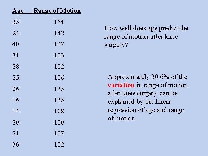
Age Range of Motion 35 154 24 142 40 137 31 133 28 122 25 126 26 135 14 108 20 120 21 127 30 122 How well does age predict the range of motion after knee surgery? Approximately 30. 6% of the variation in range of motion after knee surgery can be explained by the linear regression of age and range of motion.

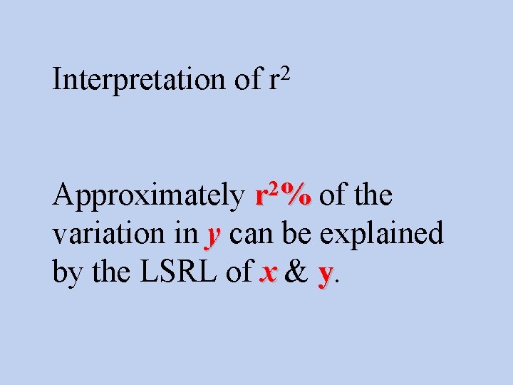
Interpretation of 2 r Approximately r 2% of the variation in y can be explained by the LSRL of x & y.

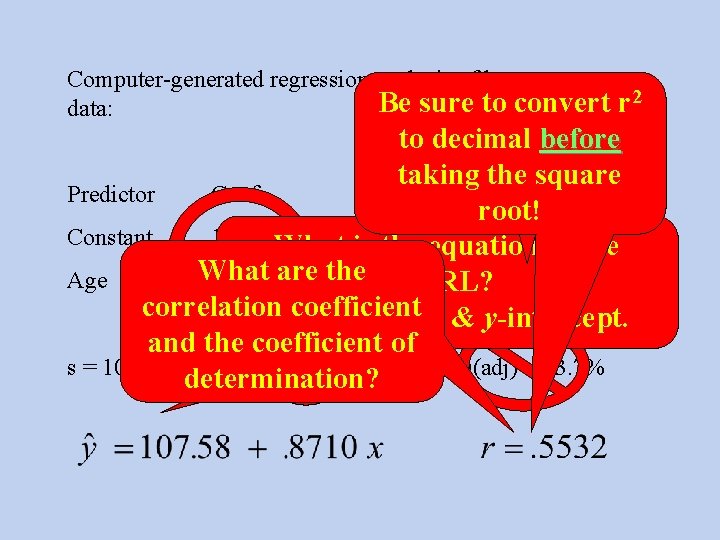
Computer-generated regression analysis of knee surgery Be sure to convert r 2 data: NEVER use to decimal before 2 adjusted r ! taking the square Predictor Coef Stdev T P root! Constant 107. 58 What is 11. 12 9. 67 of 0. 000 the equation the What Age 0. 8710 are the 0. 4146 LSRL? 2. 10 0. 062 correlation coefficient Find the slope & y-intercept. and the coefficient of s = 10. 42 R-sq = 30. 6% R-sq(adj) = 23. 7% determination?

Outlier – • In a regression setting, an outlier is a data point with a large residual

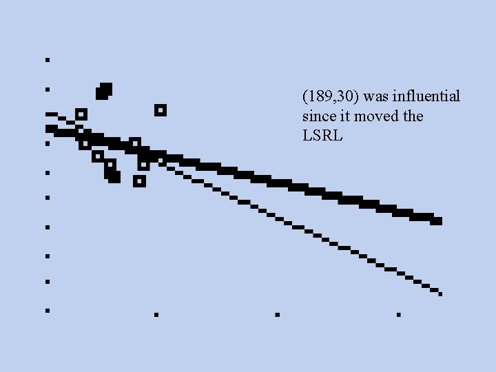
Influential point • A point that influences where the LSRL is located • If removed, it will significantly change the slope of the LSRL

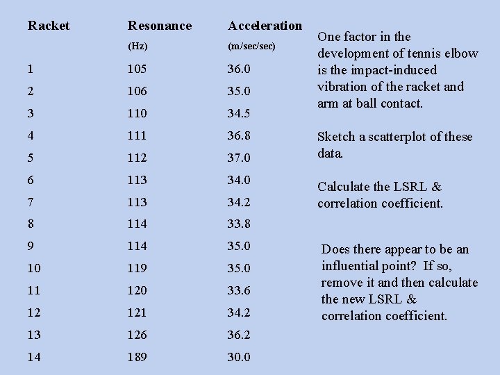
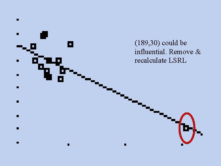
Racket Resonance Acceleration (Hz) (m/sec) 1 105 36. 0 2 106 35. 0 3 110 34. 5 4 111 36. 8 5 112 37. 0 6 113 34. 0 7 113 34. 2 8 114 33. 8 9 114 35. 0 10 119 35. 0 11 120 33. 6 12 121 34. 2 13 126 36. 2 14 189 30. 0 One factor in the development of tennis elbow is the impact-induced vibration of the racket and arm at ball contact. Sketch a scatterplot of these data. Calculate the LSRL & correlation coefficient. Does there appear to be an influential point? If so, remove it and then calculate the new LSRL & correlation coefficient.

(189, 30) could be influential. Remove & recalculate LSRL

(189, 30) was influential since it moved the LSRL

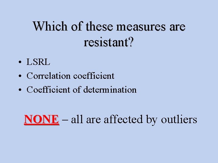
Which of these measures are resistant? • LSRL • Correlation coefficient • Coefficient of determination NONE – all are affected by outliers