Regression and Residual Plots Section 3 2 Tapping

Regression and Residual Plots Section 3. 2

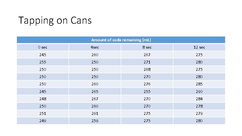
Tapping on Cans Amount of soda remaining (m. L) 0 sec 4 sec 8 sec 12 sec 245 260 267 275 250 271 280 250 268 275 250 270 280 250 260 276 285 245 265 255 290 248 267 270 284 250 260 278 251 261 275 279 249 259 275 280

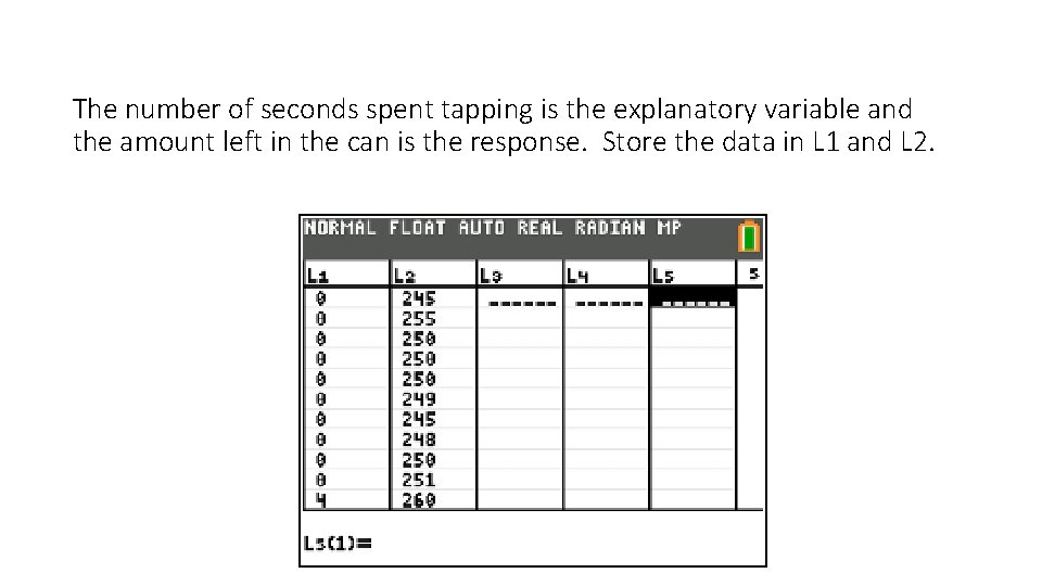
The number of seconds spent tapping is the explanatory variable and the amount left in the can is the response. Store the data in L 1 and L 2.

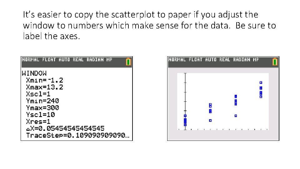
It’s easier to copy the scatterplot to paper if you adjust the window to numbers which make sense for the data. Be sure to label the axes.

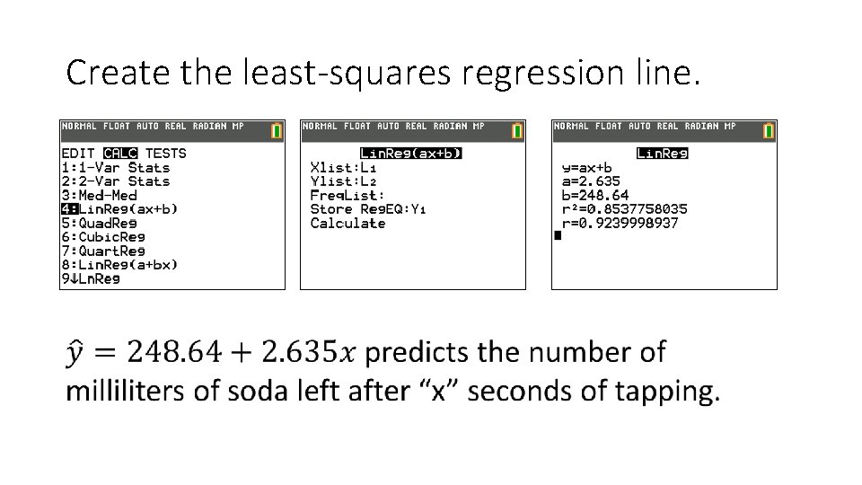
Create the least-squares regression line.

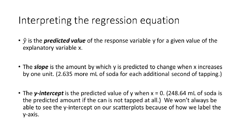
Interpreting the regression equation •

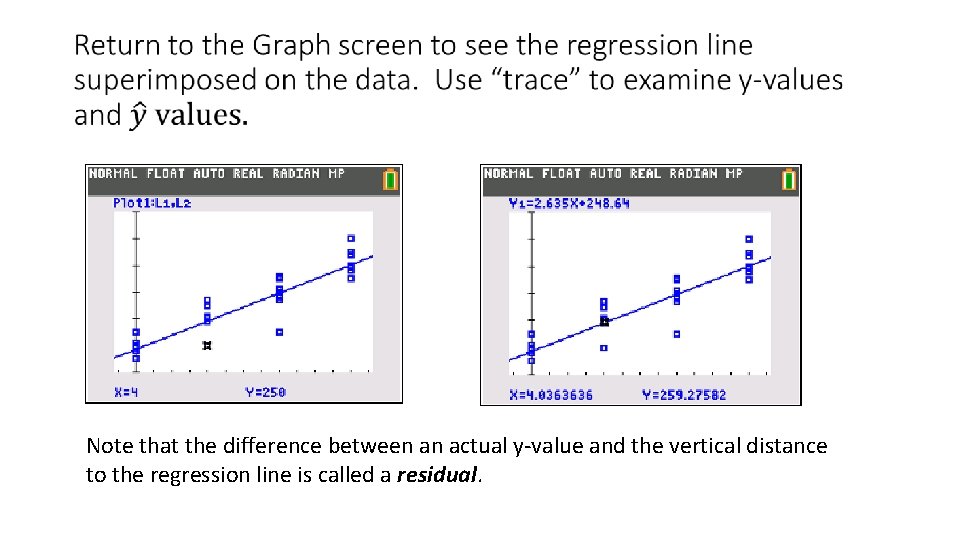
Note that the difference between an actual y-value and the vertical distance to the regression line is called a residual.

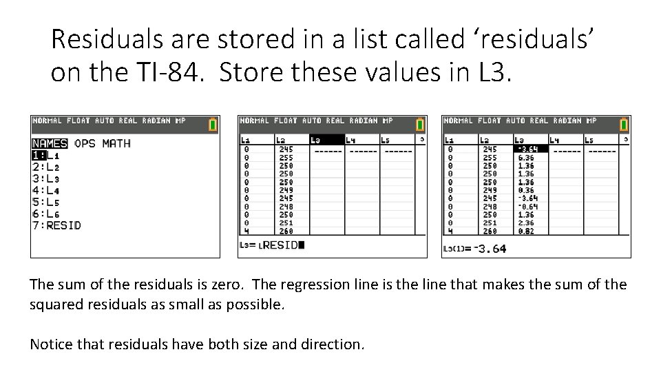
Residuals are stored in a list called ‘residuals’ on the TI-84. Store these values in L 3. The sum of the residuals is zero. The regression line is the line that makes the sum of the squared residuals as small as possible. Notice that residuals have both size and direction.

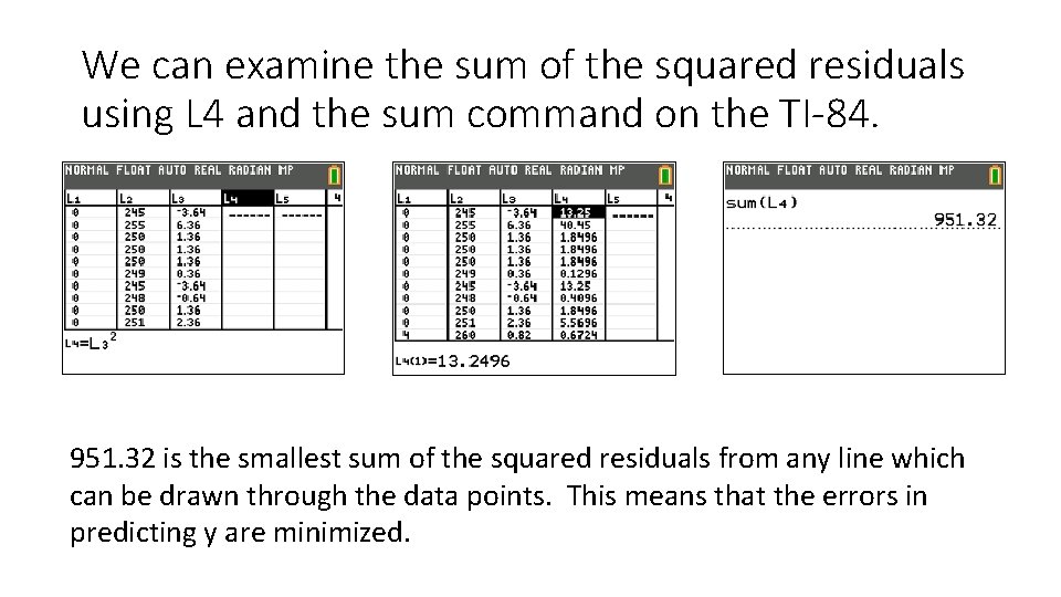
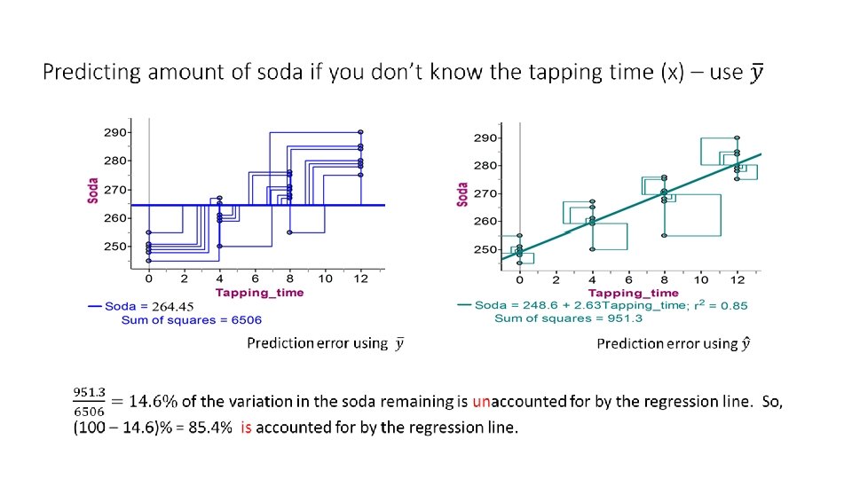
We can examine the sum of the squared residuals using L 4 and the sum command on the TI-84. 951. 32 is the smallest sum of the squared residuals from any line which can be drawn through the data points. This means that the errors in predicting y are minimized.

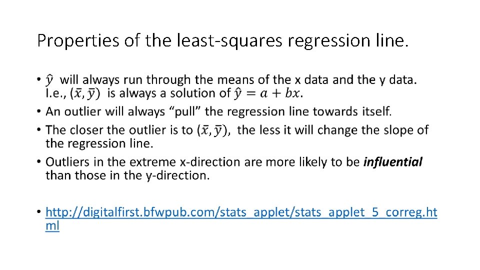
Properties of the least-squares regression line. •

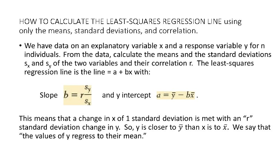
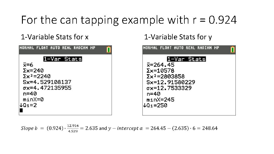
HOW TO CALCULATE THE LEAST-SQUARES REGRESSION LINE using only the means, standard deviations, and correlation. •

For the can tapping example with r = 0. 924 1 -Variable Stats for x 1 -Variable Stats for y

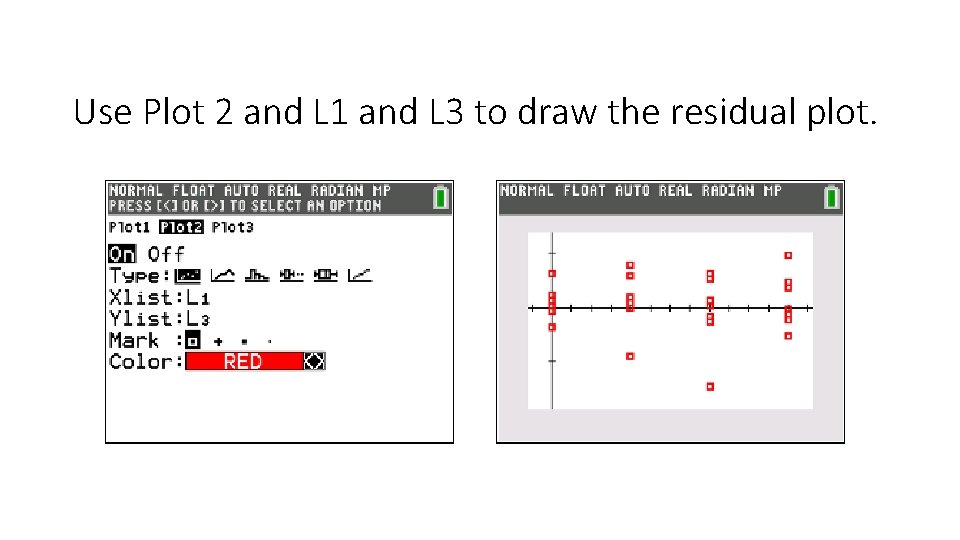
Determining the appropriateness of a linear model using a “residual plot” • Because the sum of the residuals (measured from the least-squared regression line) is always zero, the mean of these residuals is also zero. • A residual plot consists of the scatterplot of the residuals and the horizontal line y = 0. The horizontal line represents the regression line. (The regression line is a distance of 0 from itself. ) • Plot the explanatory variable values (in L 1) as x, and the residuals (in L 3) as y.

Use Plot 2 and L 1 and L 3 to draw the residual plot.

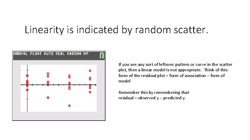
Linearity is indicated by random scatter. If you see any sort of leftover pattern or curve in the scatter plot, then a linear model is not appropriate. Think of this: form of the residual plot = form of association – form of model Remember this by remembering that residual = observed y – predicted y.

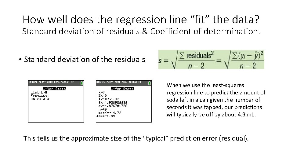
How well does the regression line “fit” the data? Standard deviation of residuals & Coefficient of determination. • Standard deviation of the residuals When we use the least-squares regression line to predict the amount of soda left in a can given the number of seconds it was tapped, our predictions will typically be off by about 4. 9 m. L. This tells us the approximate size of the “typical” prediction error (residual).

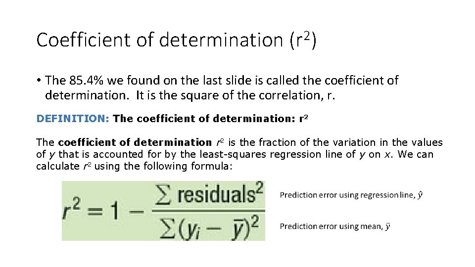
Coefficient of determination (r 2) • The 85. 4% we found on the last slide is called the coefficient of determination. It is the square of the correlation, r. DEFINITION: The coefficient of determination: r 2 The coefficient of determination r 2 is the fraction of the variation in the values of y that is accounted for by the least-squares regression line of y on x. We can calculate r 2 using the following formula:

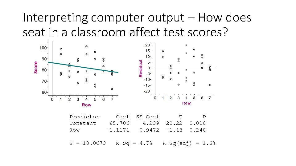
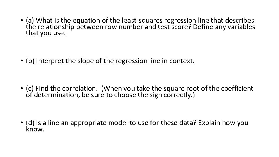
Interpreting computer output – How does seat in a classroom affect test scores? Predictor Coef SE Coef T P Constant 85. 706 4. 239 20. 22 0. 000 Row -1. 1171 0. 9472 -1. 18 0. 248 S = 10. 0673 R-Sq = 4. 7% R-Sq(adj) = 1. 3%

• (a) What is the equation of the least-squares regression line that describes the relationship between row number and test score? Define any variables that you use. • (b) Interpret the slope of the regression line in context. • (c) Find the correlation. (When you take the square root of the coefficient of determination, be sure to choose the sign correctly. ) • (d) Is a line an appropriate model to use for these data? Explain how you know.

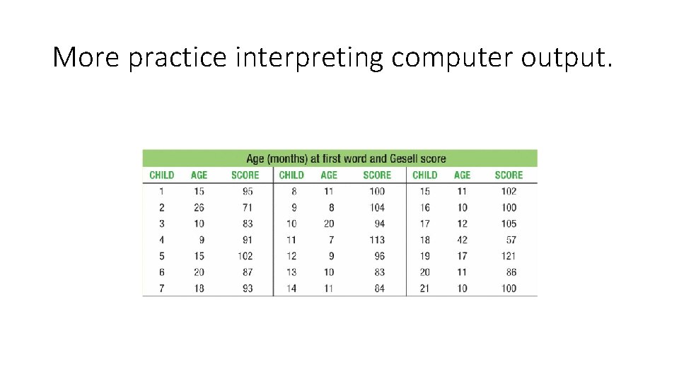
More practice interpreting computer output.

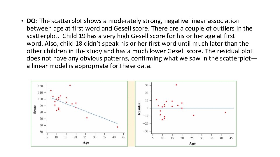
Should we use a linear model and, if so, how accurate will our predictions be? • Use the four step process: State Plan Do Conclude • STATE: Is a linear model appropriate for these data? If so, how well does the least-squares regression line fit the data? • PLAN: To determine whether a linear model is appropriate, we will look at the scatterplot and residual plot to see if the association is linear or nonlinear. Then, if a linear model is appropriate, we will use the standard deviation of the residuals and r 2 to measure how well the least-squares line fits the data.

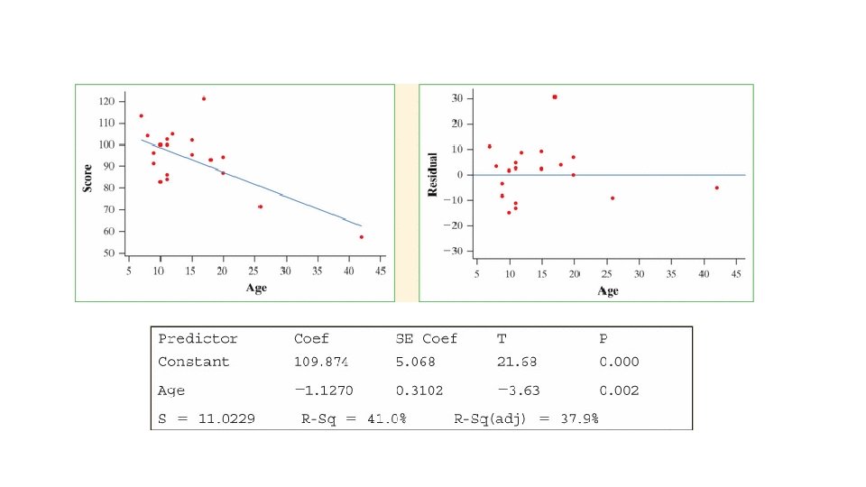
• DO: The scatterplot shows a moderately strong, negative linear association between age at first word and Gesell score. There a couple of outliers in the scatterplot. Child 19 has a very high Gesell score for his or her age at first word. Also, child 18 didn’t speak his or her first word until much later than the other children in the study and has a much lower Gesell score. The residual plot does not have any obvious patterns, confirming what we saw in the scatterplot— a linear model is appropriate for these data.

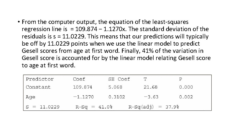
• From the computer output, the equation of the least-squares regression line is = 109. 874 − 1. 1270 x. The standard deviation of the residuals is s = 11. 0229. This means that our predictions will typically be off by 11. 0229 points when we use the linear model to predict Gesell scores from age at first word. Finally, 41% of the variation in Gesell score is accounted for by the linear model relating Gesell score to age at first word.

• CONCLUDE: Although a linear model is appropriate for these data, our predictions might not be very accurate. Our typical prediction error is about 11 points, and more than half of the variation in Gesell score is still unaccounted for. Furthermore, we should be hesitant to use this model to make predictions until we understand the effect of the two outliers on the regression results.

DEFINITION: Outliers and influential observations in regression • An outlier is an observation that lies outside the overall pattern of the other observations. Points that are outliers in the y direction but not the x direction of a scatterplot have large residuals. Other outliers may not have large residuals. • An observation is influential for a statistical calculation if removing it would markedly change the result of the calculation. Points that are outliers in the x direction of a scatterplot are often influential for the least-squares regression line. (the best way to determine if an outlier is influential is to calculate the regression line with and without the point. ) http: //digitalfirst. bfwpub. com/stats_applet_5_correg. html