Supervised 2 Linear and logistic regression 1042 Data

Supervised 2 Linear and logistic regression 1042. Data Science in Practice Week 12, 05/09 Jia-Ming Chang http: //www. cs. nccu. edu. tw/~jmchang/course/1042/datascience/ The slide isonly for educational purposes. If any infringement, please contact me, we will correct immediately.

homewrok 3 index link 1 https: //github. com/Blueswen/DSP/tree/master/Homework 3 2 https: //rplc. shinyapps. io/evaluation/ 3 https: //summer. shinyapps. io/hw 03/ 4 https: //wallyliu. shinyapps. io/Homework 3/ 5 https: //cyyang. shinyapps. io/hw 3_104753024_Chun-Yao_Yang/ 6 https: //sachitmahajan. shinyapps. io/homework 3/ 7 https: //georgekibirige-104761506. shinyapps. io/homework 3/ 8 https: //mekjr 1. shinyapps. io/hw 3_assignment/ 9 https: //kalpana. shinyapps. io/assignment/ 10 https: //tasshussain. shinyapps. io/Homework-3/ 11 https: //redwing. shinyapps. io/Homework 3/ score

Linear and logistic regression • Using linear regression to predict quantities • Using logistic regression to predict probabilities or categories • Extracting relations and advice from functional models • Interpreting the diagnostics from R’s lm() call • Interpreting the diagnostics from R’s glm() call Zumel, N. & Mount, J. Practical Data Science with R. (Manning, 2014)

Linear and logistic regression • This class of methods is especially useful when you don’t just want to predict an outcome, but you also want to know the relationship between the input variables and the outcome. • This knowledge can prove useful because this relationship can often be used as advice on how to get the outcome that you want. Zumel, N. & Mount, J. Practical Data Science with R. (Manning, 2014)

linear regression • for every person i , we want to predict pounds. lost[i] based on daily. cals[i] and daily. exercise[i] • pounds. lost[i] = b. cals * daily. cals[i] + b. exercise * daily. exercise[i] – pounds. lost[i] : dependent or response variable – daily. cals[i], daily. exercise[i] : independent or explanatory variables – b. cals, b. exercise : coefficients or betas • y[i] ~ f(x[i, ]) = b[1] x[i, 1] + b[2] x[i, 2] +. . . b[n] x[i, n] + e[i] – We want numbers b[1], . . . , b[n] (called the coefficients or betas ) such that f(x[i, ]) is as near as possible to y[i] for all (x[i, ], y[i]) pairs in our training data. – e[i] : unsystematic errors • average to 0 • uncorrelated with x[i, ] and y[i]. Zumel, N. & Mount, J. Practical Data Science with R. (Manning, 2014)

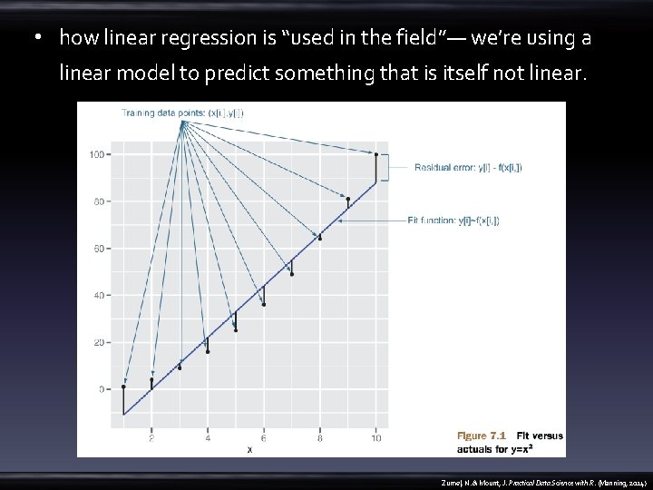
• how linear regression is “used in the field”— we’re using a linear model to predict something that is itself not linear. Zumel, N. & Mount, J. Practical Data Science with R. (Manning, 2014)

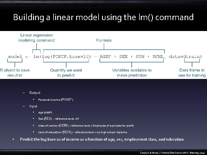
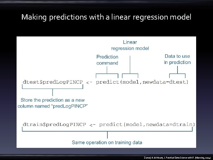
Prepare data • 2011 US Census PUMS data – predict personal income from other demographic variables such as age and education • https: //github. com/Win. Vector/zm. PDSw. R/raw/master/PUMS/psub. RData • load("psub. RData") • dtrain <- subset(psub, ORIGRANDGROUP >= 500) • dtest <- subset(psub, ORIGRANDGROUP < 500) • model <- lm(log(PINCP, base=10) ~ AGEP + SEX + COW + SCHL, data=dtrain) • dtest$pred. Log. PINCP <- predict(model, newdata=dtest) • dtrain$pred. Log. PINCP <- predict(model, newdata=dtrain) Zumel, N. & Mount, J. Practical Data Science with R. (Manning, 2014)

Building a linear model using the lm() command – Output • – • Personal income (PINCP ) Input • age (AGEP) • Sex (SEX) : reference level =M • class of worker (COW) : reference level = Employee of a private for-profit • level of education (SCHL) : reference level = no high school diploma Predict the log base 10 of income as a function of age, sex, employment class, and education. Zumel, N. & Mount, J. Practical Data Science with R. (Manning, 2014)

Making predictions with a linear regression model Zumel, N. & Mount, J. Practical Data Science with R. (Manning, 2014)

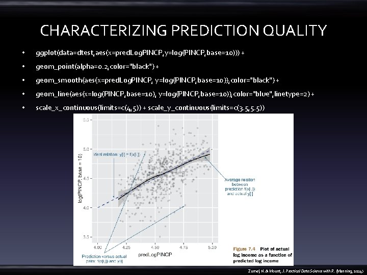
CHARACTERIZING PREDICTION QUALITY • ggplot(data=dtest, aes(x=pred. Log. PINCP, y=log(PINCP, base=10))) + • geom_point(alpha=0. 2, color="black") + • geom_smooth(aes(x=pred. Log. PINCP, y=log(PINCP, base=10)), color="black") + • geom_line(aes(x=log(PINCP, base=10), y=log(PINCP, base=10)), color="blue", linetype=2) + • scale_x_continuous(limits=c(4, 5)) + scale_y_continuous(limits=c(3. 5, 5. 5)) Zumel, N. & Mount, J. Practical Data Science with R. (Manning, 2014)

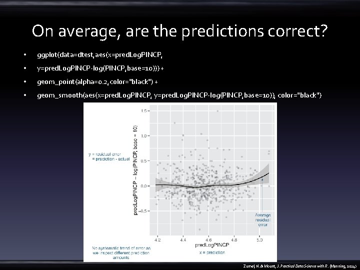
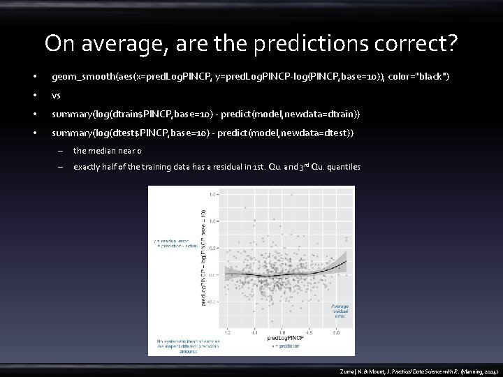
On average, are the predictions correct? • ggplot(data=dtest, aes(x=pred. Log. PINCP, • y=pred. Log. PINCP-log(PINCP, base=10))) + • geom_point(alpha=0. 2, color="black") + • geom_smooth(aes(x=pred. Log. PINCP, y=pred. Log. PINCP-log(PINCP, base=10)), color="black") Zumel, N. & Mount, J. Practical Data Science with R. (Manning, 2014)

On average, are the predictions correct? • geom_smooth(aes(x=pred. Log. PINCP, y=pred. Log. PINCP-log(PINCP, base=10)), color="black") • vs • summary(log(dtrain$PINCP, base=10) - predict(model, newdata=dtrain)) • summary(log(dtest$PINCP, base=10) - predict(model, newdata=dtest)) – the median near 0 – exactly half of the training data has a residual in 1 st. Qu. and 3 rd Qu. quantiles Zumel, N. & Mount, J. Practical Data Science with R. (Manning, 2014)

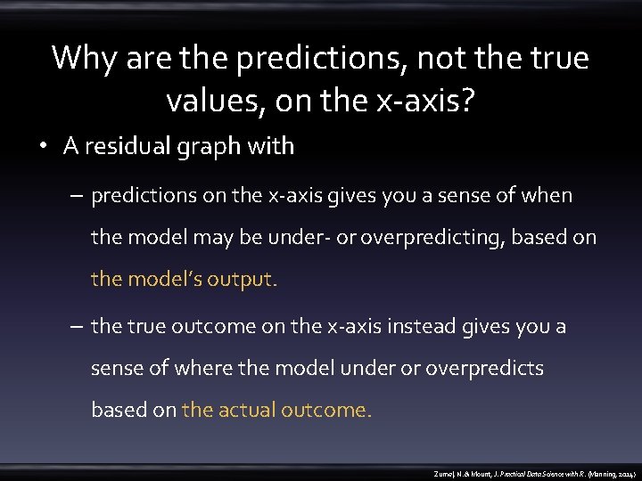
Why are the predictions, not the true values, on the x-axis? • A residual graph with – predictions on the x-axis gives you a sense of when the model may be under- or overpredicting, based on the model’s output. – the true outcome on the x-axis instead gives you a sense of where the model under or overpredicts based on the actual outcome. Zumel, N. & Mount, J. Practical Data Science with R. (Manning, 2014)

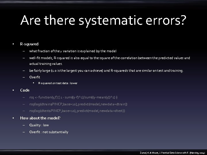
Are there systematic errors? • R-squared – what fraction of the y variation is explained by the model – well-fit models, R-squared is also equal to the square of the correlation between the predicted values and actual training values. – be fairly large (1. 0 is the largest you can achieve) and R-squareds that are similar on test and training. – Overfit • • • R-squared on test data : lower Code – rsq <- function(y, f) { 1 - sum((y-f)^2)/sum((y-mean(y))^2) } – rsq(log(dtrain$PINCP, base=10), predict(model, newdata=dtrain)) – rsq(log(dtest$PINCP, base=10), predict(model, newdata=dtest)) How about the model? – Quality : low – Overfit : not substantially Zumel, N. & Mount, J. Practical Data Science with R. (Manning, 2014)

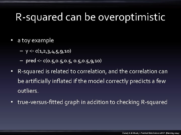
R-squared can be overoptimistic • a toy example – y <- c(1, 2, 3, 4, 5, 9, 10) – pred <- c(0. 5, 9, 10) • R-squared is related to correlation, and the correlation can be artificially inflated if the model correctly predicts a few outliers. • true-versus-fitted graph in addition to checking R-squared Zumel, N. & Mount, J. Practical Data Science with R. (Manning, 2014)

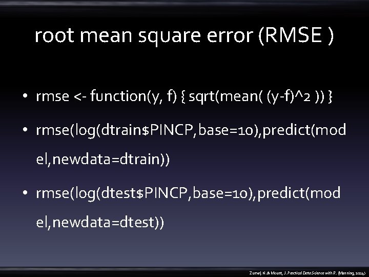
root mean square error (RMSE ) • rmse <- function(y, f) { sqrt(mean( (y-f)^2 )) } • rmse(log(dtrain$PINCP, base=10), predict(mod el, newdata=dtrain)) • rmse(log(dtest$PINCP, base=10), predict(mod el, newdata=dtest)) Zumel, N. & Mount, J. Practical Data Science with R. (Manning, 2014)

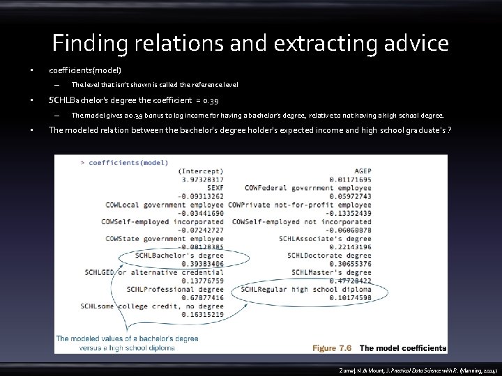
Finding relations and extracting advice • coefficients(model) – • SCHLBachelor's degree the coefficient = 0. 39 – • The level that isn’t shown is called the reference level The model gives a 0. 39 bonus to log income for having a bachelor’s degree, relative to not having a high school degree. The modeled relation between the bachelor’s degree holder’s expected income and high school graduate’s ? Zumel, N. & Mount, J. Practical Data Science with R. (Manning, 2014)

Finding relations and extracting advice • AGEP is a continuous variable with coefficient 0. 0117? – a one-year increase in age, adding a 0. 0117 bonus to log income Zumel, N. & Mount, J. Practical Data Science with R. (Manning, 2014)

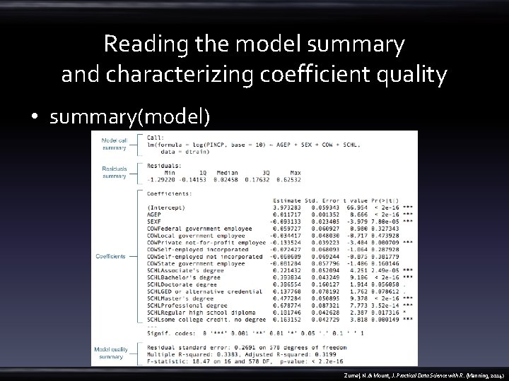
Reading the model summary and characterizing coefficient quality • summary(model) Zumel, N. & Mount, J. Practical Data Science with R. (Manning, 2014)

THE COEFFICIENTS TABLE • summary(model)$coefficients • The p-value : the probability of seeing a coefficient with a magnitude as large as we observe if the true coefficient is really 0 (if the variable has no effect on the outcome) – >=0. 05, is not to be trusted – 1 e-23 vs 1 e-08? Zumel, N. & Mount, J. Practical Data Science with R. (Manning, 2014)

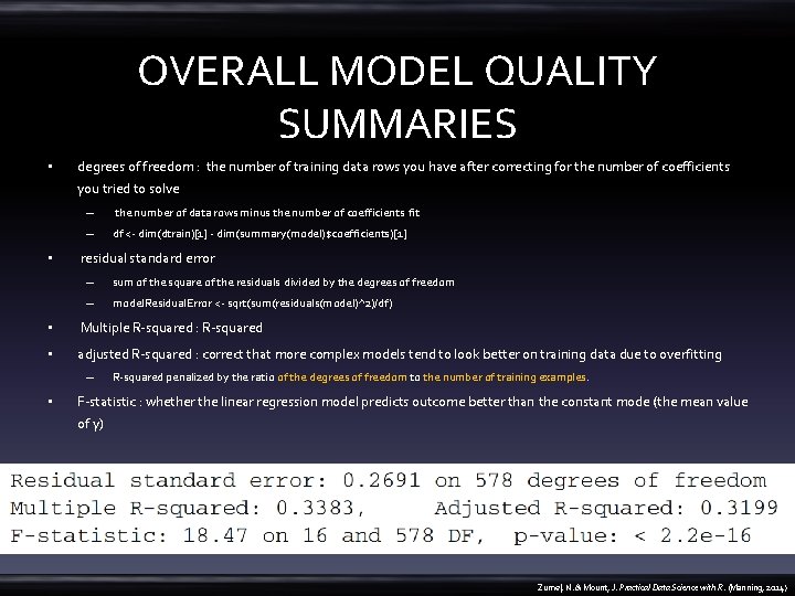
OVERALL MODEL QUALITY SUMMARIES • degrees of freedom : the number of training data rows you have after correcting for the number of coefficients you tried to solve • – the number of data rows minus the number of coefficients fit – df <- dim(dtrain)[1] - dim(summary(model)$coefficients)[1] residual standard error – sum of the square of the residuals divided by the degrees of freedom – model. Residual. Error <- sqrt(sum(residuals(model)^2)/df) • Multiple R-squared : R-squared • adjusted R-squared : correct that more complex models tend to look better on training data due to overfitting – • R-squared penalized by the ratio of the degrees of freedom to the number of training examples. F-statistic : whether the linear regression model predicts outcome better than the constant mode (the mean value of y) Zumel, N. & Mount, J. Practical Data Science with R. (Manning, 2014)

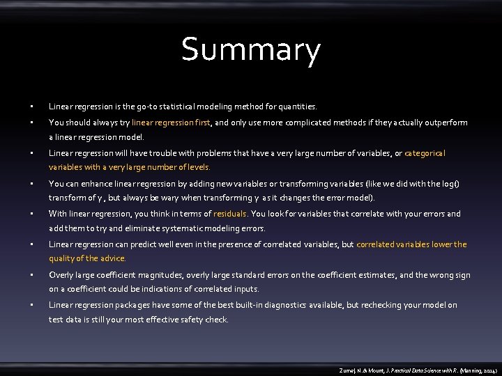
Summary • Linear regression is the go-to statistical modeling method for quantities. • You should always try linear regression first, and only use more complicated methods if they actually outperform a linear regression model. • Linear regression will have trouble with problems that have a very large number of variables, or categorical variables with a very large number of levels. • You can enhance linear regression by adding new variables or transforming variables (like we did with the log() transform of y , but always be wary when transforming y as it changes the error model). • With linear regression, you think in terms of residuals. You look for variables that correlate with your errors and add them to try and eliminate systematic modeling errors. • Linear regression can predict well even in the presence of correlated variables, but correlated variables lower the quality of the advice. • Overly large coefficient magnitudes, overly large standard errors on the coefficient estimates, and the wrong sign on a coefficient could be indications of correlated inputs. • Linear regression packages have some of the best built-in diagnostics available, but rechecking your model on test data is still your most effective safety check. Zumel, N. & Mount, J. Practical Data Science with R. (Manning, 2014)

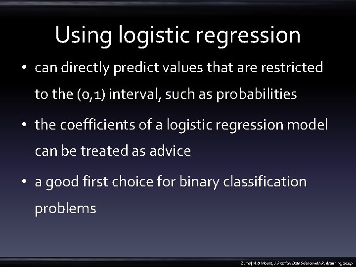
Using logistic regression • can directly predict values that are restricted to the (0, 1) interval, such as probabilities • the coefficients of a logistic regression model can be treated as advice • a good first choice for binary classification problems Zumel, N. & Mount, J. Practical Data Science with R. (Manning, 2014)

logistic regression • P[y[i] in class] ~ f(x[i, ]) = s(a+b[1] x[i, 1] +. . . b[n] x[i, n]) – s(z) = 1/(1+exp(z)), sigmoid function , maps real numbers to the interval (0, 1) – find the b[1], . . . , b[n] such that f(x[i, ]) is the best possible estimate of y[i] – inverse of the sigmoid is the logit = log of the odds = log-odds= log(p/(1 -p)) – assumes that logit(y) is linear in the values of x => as a linear regression that finds the log-odds of the probability that you’re interested in. Zumel, N. & Mount, J. Practical Data Science with R. (Manning, 2014)

Prepare data • The goal is to design a plan that provisions neonatal emergency equipment to delivery rooms. • https: //github. com/Win. Vector/zm. PDSw. R/raw/master/ CDC/Natal. Risk. Data. r. Data • load("Natal. Risk. Data. r. Data") • train <- sdata[sdata$ORIGRANDGROUP<=5, ] • test <- sdata[sdata$ORIGRANDGROUP>5, ] Zumel, N. & Mount, J. Practical Data Science with R. (Manning, 2014)

variables in natality dataset Variable Type Description at. Risk Logical TRUE if 5 -minute Apgar score < 7; FALSE otherwise PWGT Numeric Mother’s prepregnancy weight UPREVIS Numeric Number of prenatal medical visits UPREVIS Logical TRUE if smoker; FALSE otherwise GESTREC 3 Categorical Two categories: <37 weeks (premature) and >=37 weeks DPLURAL Categorical Birth plurality, three categories: single/twin/triplet+ ULD_MECO Logical TRUE if moderate/heavy fecal staining of amniotic fluid ULD_PRECIP Logical TRUE for unusually short labor (< three hours) ULD_BREECH Logical TRUE for breech (pelvis first) birth position URF_DIAB Logical TRUE if mother is diabetic URF_CHYPER Logical TRUE if mother has chronic hypertension URF_PHYPER Logical TRUE if mother has pregnancy-related hypertension URF_ECLAM Logical TRUE if mother experienced eclampsia: pregnancyrelated seizures Zumel, N. & Mount, J. Practical Data Science with R. (Manning, 2014)

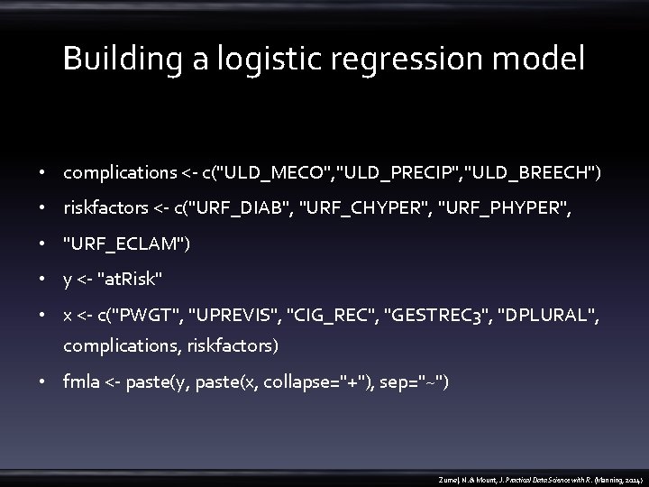
Building a logistic regression model • complications <- c("ULD_MECO", "ULD_PRECIP", "ULD_BREECH") • riskfactors <- c("URF_DIAB", "URF_CHYPER", "URF_PHYPER", • "URF_ECLAM") • y <- "at. Risk" • x <- c("PWGT", "UPREVIS", "CIG_REC", "GESTREC 3", "DPLURAL", complications, riskfactors) • fmla <- paste(y, paste(x, collapse="+"), sep="~") Zumel, N. & Mount, J. Practical Data Science with R. (Manning, 2014)

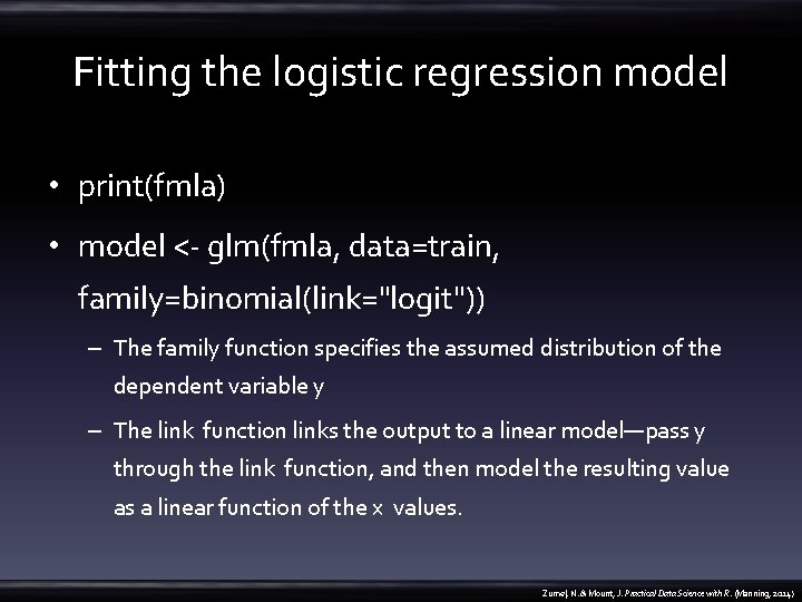
Fitting the logistic regression model • print(fmla) • model <- glm(fmla, data=train, family=binomial(link="logit")) – The family function specifies the assumed distribution of the dependent variable y – The link function links the output to a linear model—pass y through the link function, and then model the resulting value as a linear function of the x values. Zumel, N. & Mount, J. Practical Data Science with R. (Manning, 2014)

Making predictions • train$pred <- predict(model, newdata=train, type="response") • test$pred <- predict(model, newdata=test, type="response") – type="response” : tells the predict() function to return the predicted probabilities y – default predict() will return the output of the link function, logit(y) • One strength of logistic regression is that it preserves the marginal probabilities of the training data. – sum up the predicted probability scores for the entire training set = the number of positive outcomes in the training set Zumel, N. & Mount, J. Practical Data Science with R. (Manning, 2014)

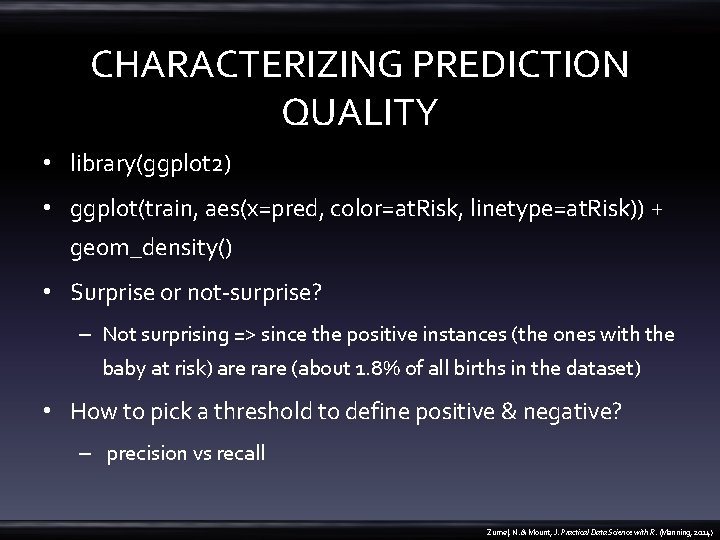
CHARACTERIZING PREDICTION QUALITY • library(ggplot 2) • ggplot(train, aes(x=pred, color=at. Risk, linetype=at. Risk)) + geom_density() • Surprise or not-surprise? – Not surprising => since the positive instances (the ones with the baby at risk) are rare (about 1. 8% of all births in the dataset) • How to pick a threshold to define positive & negative? – precision vs recall Zumel, N. & Mount, J. Practical Data Science with R. (Manning, 2014)

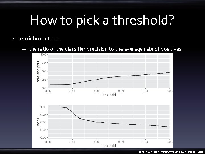
How to pick a threshold? • enrichment rate – the ratio of the classifier precision to the average rate of positives Zumel, N. & Mount, J. Practical Data Science with R. (Manning, 2014)

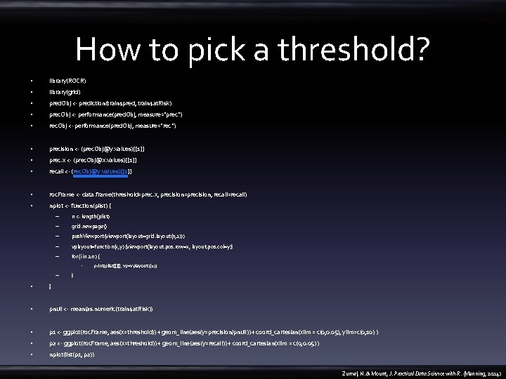
How to pick a threshold? • library(ROCR) • library(grid) • pred. Obj <- prediction(train$pred, train$at. Risk) • prec. Obj <- performance(pred. Obj, measure="prec") • rec. Obj <- performance(pred. Obj, measure="rec") • precision <- (prec. Obj@y. values)[[1]] • prec. x <- (prec. Obj@x. values)[[1]] • recall <- (rec. Obj@y. values)[[1]] • roc. Frame <- data. frame(threshold=prec. x, precision=precision, recall=recall) • nplot <- function(plist) { – n <- length(plist) – grid. newpage() – push. Viewport(viewport(layout=grid. layout(n, 1))) – vplayout=function(x, y) {viewport(layout. pos. row=x, layout. pos. col=y)} – for(i in 1: n) { – } • print(plist[[i]], vp=vplayout(i, 1)) • } • pnull <- mean(as. numeric(train$at. Risk)) • p 1 <- ggplot(roc. Frame, aes(x=threshold)) + geom_line(aes(y=precision/pnull)) + coord_cartesian(xlim = c(0, 0. 05), ylim=c(0, 10) ) • p 2 <- ggplot(roc. Frame, aes(x=threshold)) + geom_line(aes(y=recall)) + coord_cartesian(xlim = c(0, 0. 05) ) • nplot(list(p 1, p 2)) Zumel, N. & Mount, J. Practical Data Science with R. (Manning, 2014)

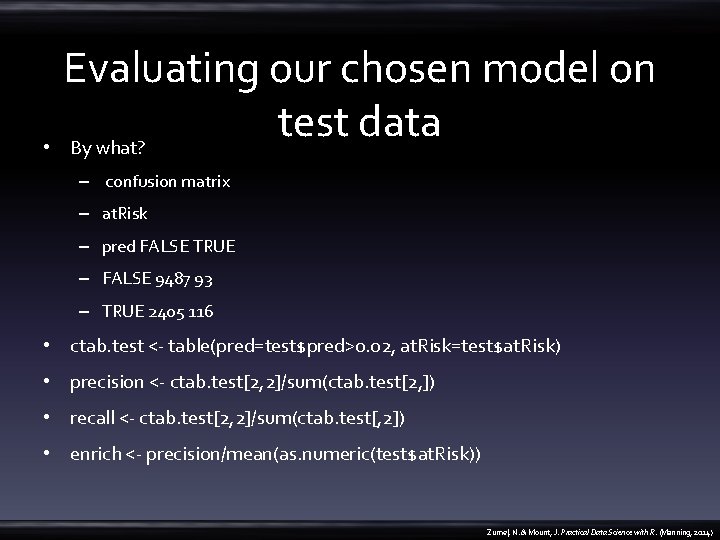
Evaluating our chosen model on test data • By what? – confusion matrix – at. Risk – pred FALSE TRUE – FALSE 9487 93 – TRUE 2405 116 • ctab. test <- table(pred=test$pred>0. 02, at. Risk=test$at. Risk) • precision <- ctab. test[2, 2]/sum(ctab. test[2, ]) • recall <- ctab. test[2, 2]/sum(ctab. test[, 2]) • enrich <- precision/mean(as. numeric(test$at. Risk)) Zumel, N. & Mount, J. Practical Data Science with R. (Manning, 2014)

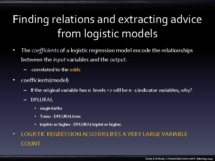
Finding relations and extracting advice from logistic models • The coefficients of a logistic regression model encode the relationships between the input variables and the output. – correlated to the odds • coefficients(model) – If the original variable has n levels => will be n -1 indicator variables, why? – DPLURAL • single births • Twins : DPLURALtwin • triplets or higher : DPLURALtriplet or higher. • LOGISTIC REGRESSION ALSO DISLIKES A VERY LARGE VARIABLE COUNT Zumel, N. & Mount, J. Practical Data Science with R. (Manning, 2014)

How to INTERPRETING THE COEFFICIENTS 1? • The coefficient for GESTREC 3< 37 = 1. 545183 – the odds of being at risk = exp(1. 545183)=4. 68883 – a full-term baby with certain characteristics has a 1% probability of being at risk • odds are p/(1 -p) , or 0. 01/0. 99 = 0. 0101 – The odds for a premature baby with the same characteristics = 0. 0101*4. 68883 = 0. 047 – a probability of being at risk of odds/(1+odds) = 0. 047/1. 047=~4. 5%. Zumel, N. & Mount, J. Practical Data Science with R. (Manning, 2014)

How to INTERPRETING THE COEFFICIENTS 2? • The coefficient for UPREVIS (number of prenatal medical visits) = -0. 06 – the odds of being at risk = exp(-0. 06)= 0. 94 – Suppose the mother of our premature baby had made no prenatal visits – a baby in the same situation whose mother had made three prenatal visits • odds of being at risk = 0. 047 * 0. 94 = 0. 039 • a probability of being at risk = 0. 039/1. 039 = 3. 75%. Zumel, N. & Mount, J. Practical Data Science with R. (Manning, 2014)

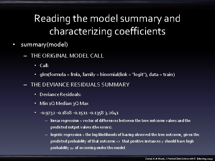
Reading the model summary and characterizing coefficients • summary(model) – THE ORIGINAL MODEL CALL • Call: • glm(formula = fmla, family = binomial(link = "logit"), data = train) – THE DEVIANCE RESIDUALS SUMMARY • Deviance Residuals: • Min 1 Q Median 3 Q Max • -0. 9732 -0. 1818 -0. 1511 -0. 1358 3. 2641 – linear regression = vector of differences between the true outcome values and the predicted output values (the errors). – logistic regression = the log likelihoods of having observed the true outcome, given the predicted probability of that outcome => that positive instances y should have high probability py of occurring under the model Zumel, N. & Mount, J. Practical Data Science with R. (Manning, 2014)

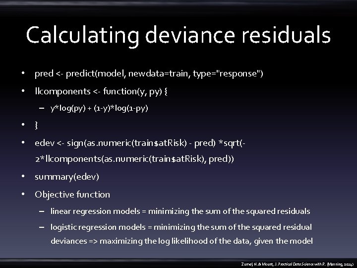
Calculating deviance residuals • pred <- predict(model, newdata=train, type="response") • llcomponents <- function(y, py) { – y*log(py) + (1 -y)*log(1 -py) • } • edev <- sign(as. numeric(train$at. Risk) - pred) *sqrt(2*llcomponents(as. numeric(train$at. Risk), pred)) • summary(edev) • Objective function – linear regression models = minimizing the sum of the squared residuals – logistic regression models = minimizing the sum of the squared residual deviances => maximizing the log likelihood of the data, given the model Zumel, N. & Mount, J. Practical Data Science with R. (Manning, 2014)

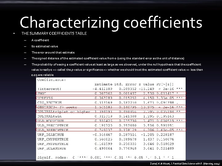
• Characterizing coefficients THE SUMMARY COEFFICIENTS TABLE – A coefficient – Its estimated value – The error around that estimate – The signed distance of the estimated coefficient value from 0 (using the standard error as the unit of distance) – The probability of seeing a coefficient value at least as large as we observed, under the null hypothesis that the coefficient value is really 0 => called the p-value or significance => whether we should trust the estimated coefficient value => less than 0. 05 are reliable Zumel, N. & Mount, J. Practical Data Science with R. (Manning, 2014)

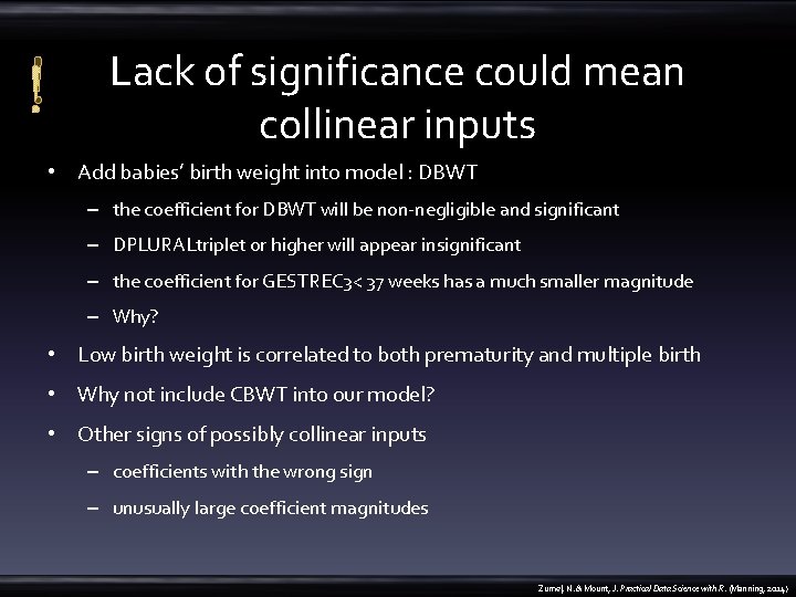
！ Lack of significance could mean collinear inputs • Add babies’ birth weight into model : DBWT – the coefficient for DBWT will be non-negligible and significant – DPLURALtriplet or higher will appear insignificant – the coefficient for GESTREC 3< 37 weeks has a much smaller magnitude – Why? • Low birth weight is correlated to both prematurity and multiple birth • Why not include CBWT into our model? • Other signs of possibly collinear inputs – coefficients with the wrong sign – unusually large coefficient magnitudes Zumel, N. & Mount, J. Practical Data Science with R. (Manning, 2014)

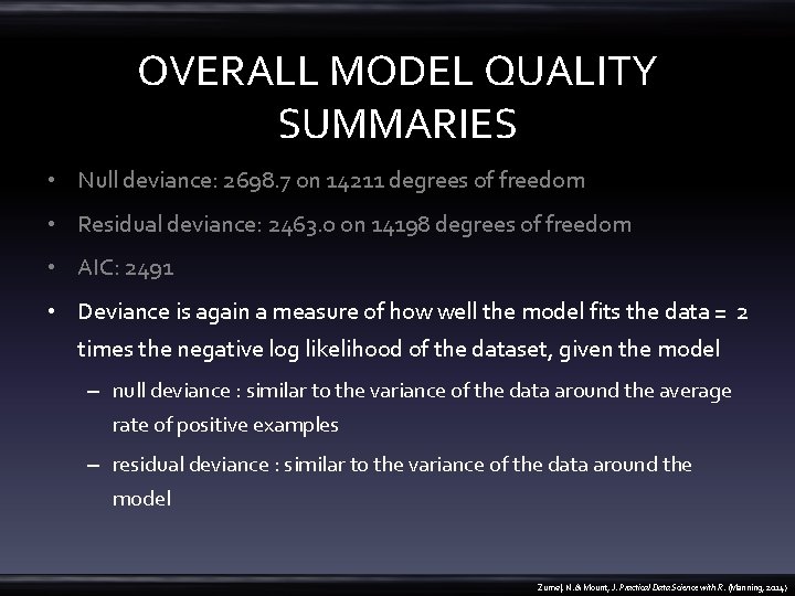
OVERALL MODEL QUALITY SUMMARIES • Null deviance: 2698. 7 on 14211 degrees of freedom • Residual deviance: 2463. 0 on 14198 degrees of freedom • AIC: 2491 • Deviance is again a measure of how well the model fits the data = 2 times the negative log likelihood of the dataset, given the model – null deviance : similar to the variance of the data around the average rate of positive examples – residual deviance : similar to the variance of the data around the model Zumel, N. & Mount, J. Practical Data Science with R. (Manning, 2014)

Computing deviance • loglikelihood <- function(y, py) { – sum(y * log(py) + (1 -y)*log(1 - py)) • } • pnull <- mean(as. numeric(train$at. Risk)) • null. dev <- -2*loglikelihood(as. numeric(train$at. Risk), pnull) • null. dev • model$null. deviance • pred <- predict(model, newdata=train, type="response") • resid. dev <- -2*loglikelihood(as. numeric(train$at. Risk), pred) • resid. dev • model$deviance • testy <- as. numeric(test$at. Risk) • testpred <- predict(model, newdata=test, type="response") • pnull. test <- mean(testy) • null. dev. test <- -2*loglikelihood(testy, pnull. test) • resid. dev. test <- -2*loglikelihood(testy, testpred) Zumel, N. & Mount, J. Practical Data Science with R. (Manning, 2014)

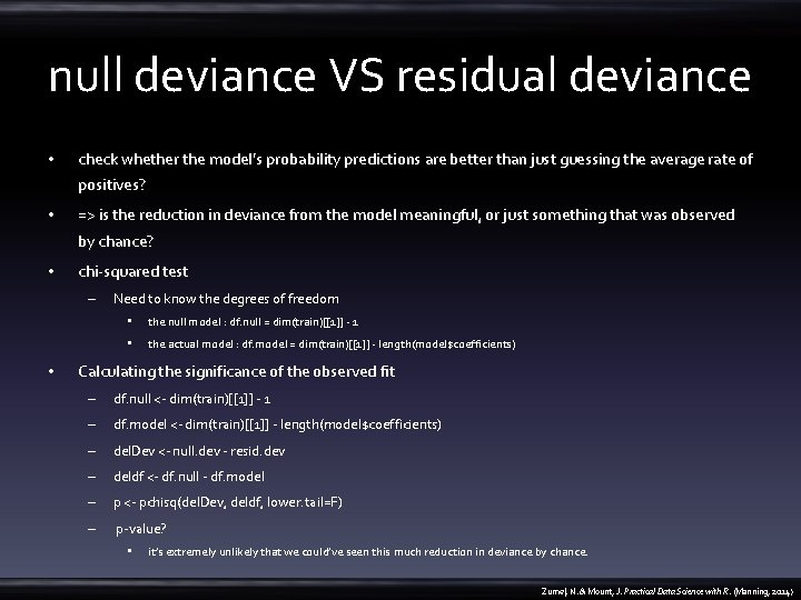
null deviance VS residual deviance • check whether the model’s probability predictions are better than just guessing the average rate of positives? • => is the reduction in deviance from the model meaningful, or just something that was observed by chance? • chi-squared test – • Need to know the degrees of freedom • the null model : df. null = dim(train)[[1]] - 1 • the actual model : df. model = dim(train)[[1]] - length(model$coefficients) Calculating the significance of the observed fit – df. null <- dim(train)[[1]] - 1 – df. model <- dim(train)[[1]] - length(model$coefficients) – del. Dev <- null. dev - resid. dev – deldf <- df. null - df. model – p <- pchisq(del. Dev, deldf, lower. tail=F) – p-value? • it’s extremely unlikely that we could’ve seen this much reduction in deviance by chance. Zumel, N. & Mount, J. Practical Data Science with R. (Manning, 2014)

The pseudo R-squared • 1 - (dev. model/dev. null) • how much of the deviance is “explained” by the model => ideal, be close to 1 • pr 2 <- 1 -(resid. dev/null. dev) • pr 2. test <- 1 -(resid. dev. test/null. dev. test) • Highly predictive model or not? – The model only explains about 7. 7– 8. 7% of the deviance => not a highly predictive model (you should have suspected that already, from figure 7. 9). – => we haven’t yet identified all the factors that actually predict at-risk births. Zumel, N. & Mount, J. Practical Data Science with R. (Manning, 2014)

P-value & The pseudo R-squared • The good p-value but the poor pseudo R-squared – The good p-value => the model is legitimate, it gives us more information than the average rate of at-risk births does alone. – The poor pseudo R-squared => the model isn’t giving us enough information to predict at-risk births with high reliability. • A bad p-vlaue but a good pseudo R-squared (on the training data) – an indication of overfit • it’s a good idea to check both • check the pseudo R-squared of the model on both training and test data. Zumel, N. & Mount, J. Practical Data Science with R. (Manning, 2014)

Akaike information criterion (AIC) • the log likelihood adjusted for the number of coefficients ~ the Rsquared of a linear regression is generally higher when the number of variables is high • aic <- 2*(length(model$coefficients) - loglikelihood(as. numeric(train$at. Risk), pred)) • decide which and how many input variables to use in the model – train many different models with different sets of variables on the same training set => the model with the lowest AIC to be the best fit Zumel, N. & Mount, J. Practical Data Science with R. (Manning, 2014)

FISHER SCORING ITERATIONS • an iterative optimization method that glm() uses to find the best coefficients for the logistic regression model • You should expect it to converge in about 6~8 iterations. – If there are more iterations than that, then the algorithm may not have converged, and the model may not be valid. Zumel, N. & Mount, J. Practical Data Science with R. (Manning, 2014)

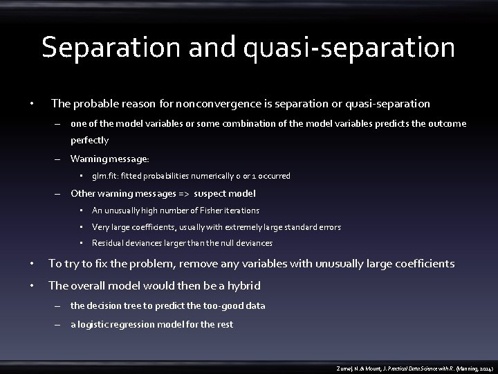
Separation and quasi-separation • The probable reason for nonconvergence is separation or quasi-separation – one of the model variables or some combination of the model variables predicts the outcome perfectly – Warning message: • glm. fit: fitted probabilities numerically 0 or 1 occurred – Other warning messages => suspect model • An unusually high number of Fisher iterations • Very large coefficients, usually with extremely large standard errors • Residual deviances larger than the null deviances • To try to fix the problem, remove any variables with unusually large coefficients • The overall model would then be a hybrid – the decision tree to predict the too-good data – a logistic regression model for the rest Zumel, N. & Mount, J. Practical Data Science with R. (Manning, 2014)

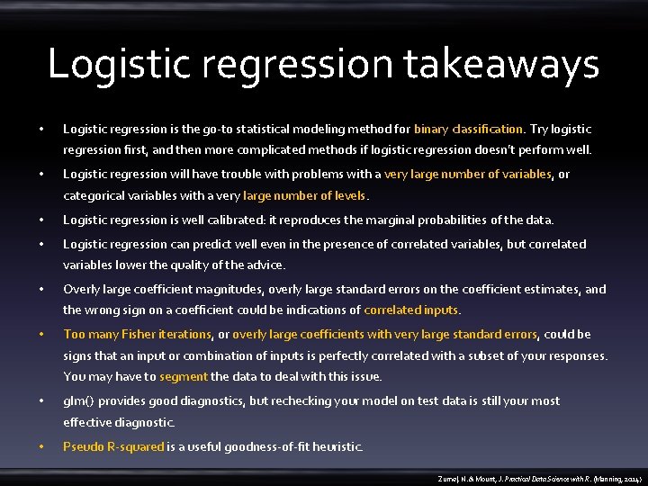
Logistic regression takeaways • Logistic regression is the go-to statistical modeling method for binary classification. Try logistic regression first, and then more complicated methods if logistic regression doesn’t perform well. • Logistic regression will have trouble with problems with a very large number of variables, or categorical variables with a very large number of levels. • Logistic regression is well calibrated: it reproduces the marginal probabilities of the data. • Logistic regression can predict well even in the presence of correlated variables, but correlated variables lower the quality of the advice. • Overly large coefficient magnitudes, overly large standard errors on the coefficient estimates, and the wrong sign on a coefficient could be indications of correlated inputs. • Too many Fisher iterations, or overly large coefficients with very large standard errors, could be signs that an input or combination of inputs is perfectly correlated with a subset of your responses. You may have to segment the data to deal with this issue. • glm() provides good diagnostics, but rechecking your model on test data is still your most effective diagnostic. • Pseudo R-squared is a useful goodness-of-fit heuristic. Zumel, N. & Mount, J. Practical Data Science with R. (Manning, 2014)

Key takeaways • Functional models allow you to better explore how changes in inputs affect predictions. • Linear regression is a good first technique for modeling quantities. • Logistic regression is good first technique for modeling probabilities. • Models with simple forms come with very powerful summaries and diagnostics. Zumel, N. & Mount, J. Practical Data Science with R. (Manning, 2014)

Any Question?