Homework Residuals Worksheet WarmUp Residuals The fit of

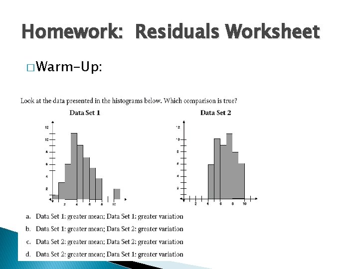
Homework: Residuals Worksheet � Warm-Up:

Residuals � The fit of a linear function to a set of data can be assessed by analyzing residuals. �A residual is the vertical distance between an observed data value and an estimated data value on a line of best fit.

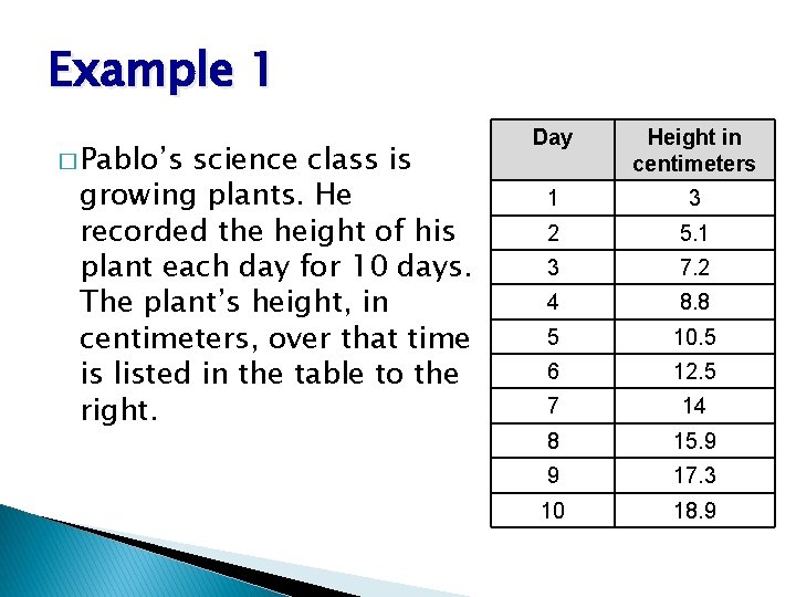
Example 1 � Pablo’s science class is growing plants. He recorded the height of his plant each day for 10 days. The plant’s height, in centimeters, over that time is listed in the table to the right. Day Height in centimeters 1 3 2 5. 1 3 7. 2 4 8. 8 5 10. 5 6 12. 5 7 14 8 15. 9 9 17. 3 10 18. 9

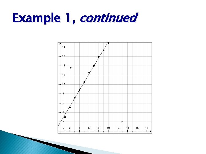
Example 1, continued • Pablo determines that the function y = 1. 73 x + 1. 87 is a good fit for the data. How close is his estimate to the actual data? Approximately how much does the plant grow each day?

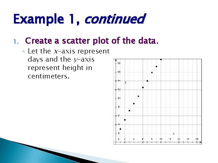
Example 1, continued 1. Create a scatter plot of the data. ◦ Let the x-axis represent days and the y-axis represent height in centimeters.

Example 1, continued 2. Draw the line of best fit through two of the data points. ◦ A good line of best fit will have some points below the line and some above the line. Use the graph to initially determine if the function is a good fit for the data.

Example 1, continued

Example 1, continued 3. Find the residuals for each data point. ◦ The residual for each data point is the difference between the observed value and the estimated value using a line of best fit. Evaluate the equation of the line at each value of x.

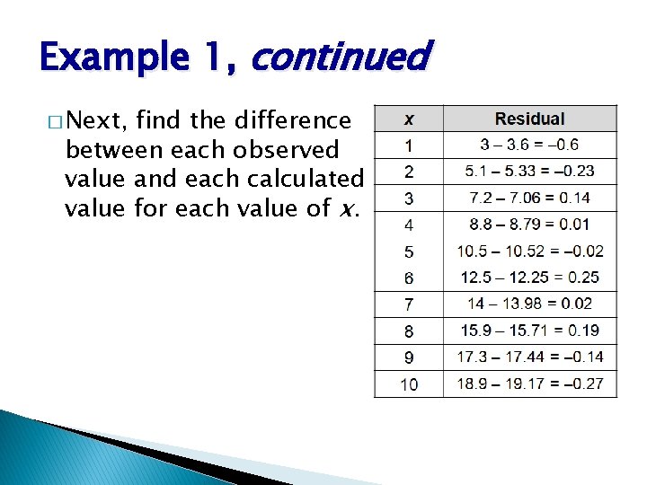
What should our values have been based on the equation? x y = 1. 73 x + 1. 87 1 y = 1. 73(1) + 1. 87 = 3. 6 2 y = 1. 73(2) + 1. 87 = 5. 33 3 y = 1. 73(3) + 1. 87 = 7. 06 4 y = 1. 73(4) + 1. 87 = 8. 79 5 y = 1. 73(5) + 1. 87 = 10. 52 6 y = 1. 73(6) + 1. 87 = 12. 25 7 y = 1. 73(7) + 1. 87 =13. 98 8 y = 1. 73(8) + 1. 87 = 15. 71 9 y = 1. 73(9) + 1. 87 = 17. 44 10 y = 1. 73(10) + 1. 87 = 19. 17

Example 1, continued � Next, find the difference between each observed value and each calculated value for each value of x.

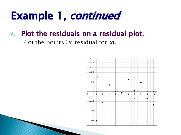
Example 1, continued 4. Plot the residuals on a residual plot. ◦ Plot the points (x, residual for x).

Example 1, continued 5. Describe the fit of the line based on the shape of the residual plot. ◦ The plot of the residuals appears to be random, with some negative and some positive values. This indicates that the line is a good line of fit.

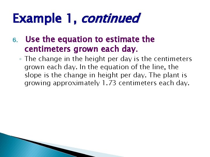
Example 1, continued 6. Use the equation to estimate the centimeters grown each day. ◦ The change in the height per day is the centimeters grown each day. In the equation of the line, the slope is the change in height per day. The plant is growing approximately 1. 73 centimeters each day.

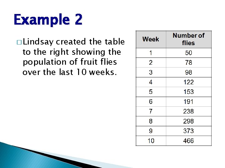
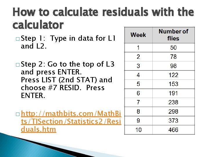
Example 2 � Lindsay created the table to the right showing the population of fruit flies over the last 10 weeks.

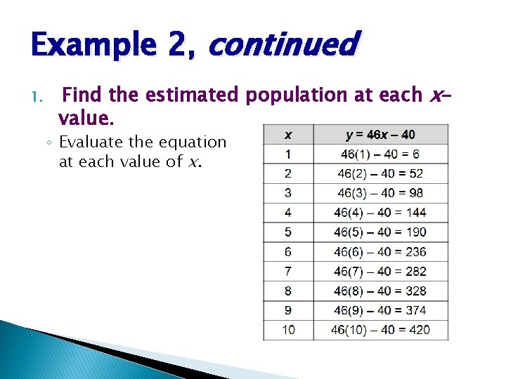
Example 2, continued � She estimates that the population of fruit flies can be represented by the equation y = 46 x – 40. Using residuals, determine if her representation is a good estimate.

Example 2, continued 1. Find the estimated population at each xvalue. ◦ Evaluate the equation at each value of x.

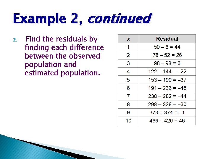
Example 2, continued 2. Find the residuals by finding each difference between the observed population and estimated population.

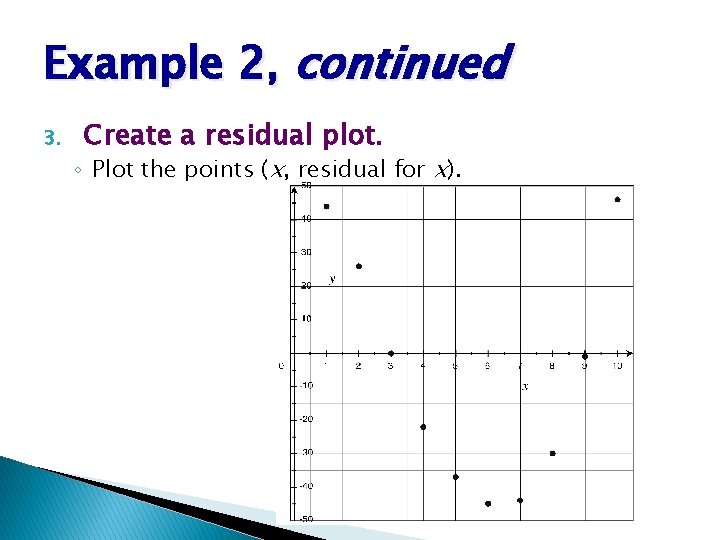
Example 2, continued 3. Create a residual plot. ◦ Plot the points (x, residual for x).

Example 2, continued 4. Analyze the residual plot to determine if the equation is a good estimate for the population. ◦ The residual plot has a U-shape. This indicates that a non-linear estimation would be a better fit for this data set. ◦ The shape of the residual plot indicates that the equation y = 46 x – 40 is not a good estimate for this data set.

How to calculate residuals with the calculator � Step 1: Type in data for L 1 and L 2. � Step 2: Go to the top of L 3 and press ENTER. Press LIST (2 nd STAT) and choose #7 RESID. Press ENTER. � http: //mathbits. com/Math. Bi ts/TISection/Statistics 2/Resi duals. htm