Residuals and Residual Plots How close is the

Residuals and Residual Plots

How close is the Line of Best Fit? • One additional method to determine if a linear model is appropriate for a data set is to analyze the residuals. • Do this by comparing the actual data point to the predicted outcome using the equation • A residual is the vertical distance between an observed data value and its predicted value using the regression equation. • A residual plot is a scatter plot of the independent variable on the x-axis and the residuals on the y-axis. The Residual Value is the difference between the actual observed value and the value predicted by the equation Residual value = observed value – predicted value

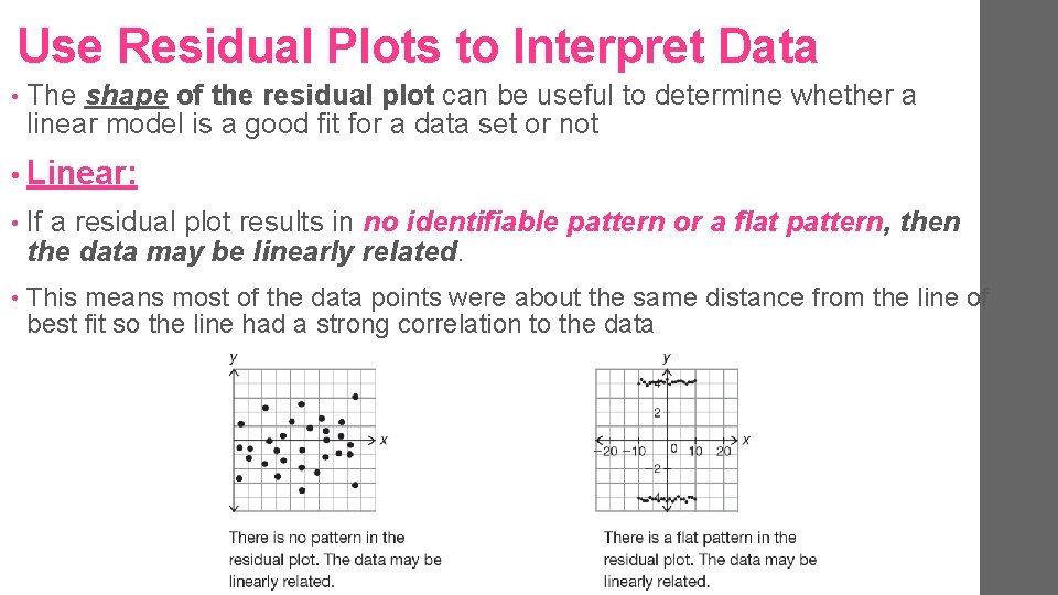
Use Residual Plots to Interpret Data • The shape of the residual plot can be useful to determine whether a linear model is a good fit for a data set or not • Linear: • If a residual plot results in no identifiable pattern or a flat pattern, then the data may be linearly related. • This means most of the data points were about the same distance from the line of best fit so the line had a strong correlation to the data

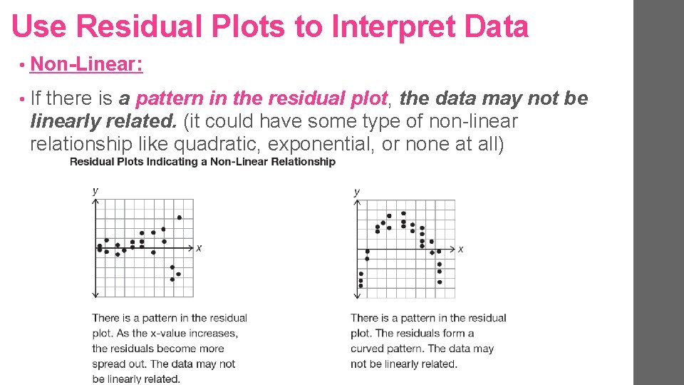
Use Residual Plots to Interpret Data • Non-Linear: • If there is a pattern in the residual plot, the data may not be linearly related. (it could have some type of non-linear relationship like quadratic, exponential, or none at all)

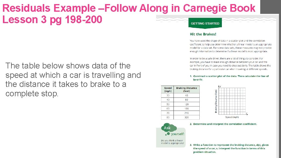
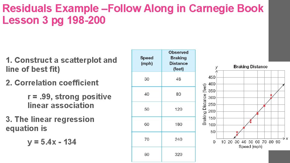
Residuals Example –Follow Along in Carnegie Book Lesson 3 pg 198 -200 The table below shows data of the speed at which a car is travelling and the distance it takes to brake to a complete stop.

Residuals Example –Follow Along in Carnegie Book Lesson 3 pg 198 -200 1. Construct a scatterplot and line of best fit) 2. Correlation coefficient r =. 99, strong positive linear association 3. The linear regression equation is y = 5. 4 x - 134

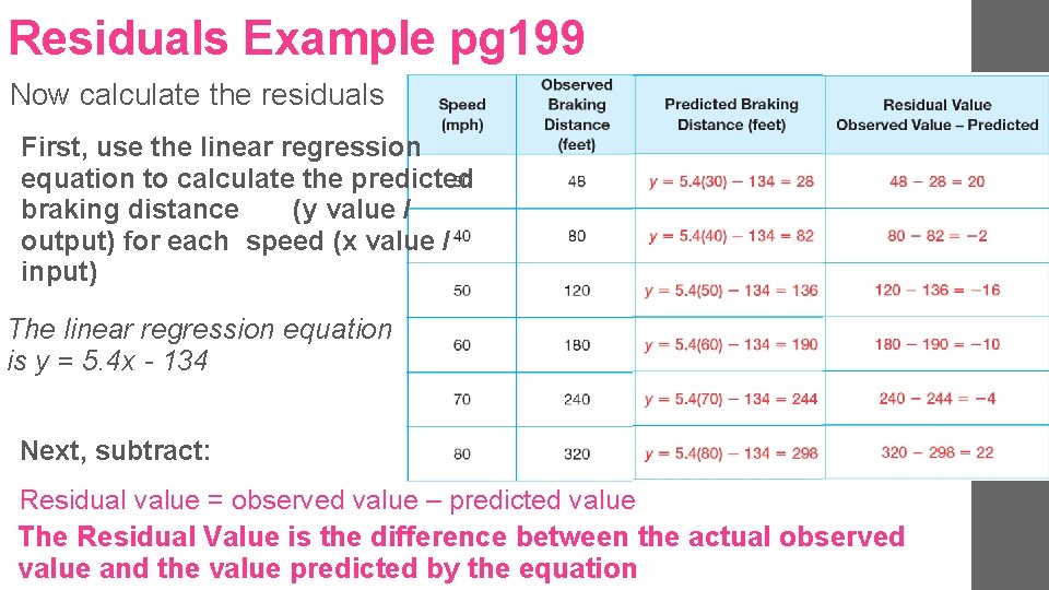
Residuals Example pg 199 Now calculate the residuals First, use the linear regression equation to calculate the predicted braking distance (y value / output) for each speed (x value / input) The linear regression equation is y = 5. 4 x - 134 Next, subtract: Residual value = observed value – predicted value The Residual Value is the difference between the actual observed value and the value predicted by the equation

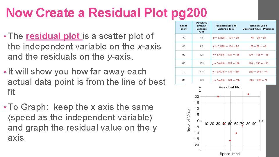
Now Create a Residual Plot pg 200 • The residual plot is a scatter plot of the independent variable on the x-axis and the residuals on the y-axis. • It will show you how far away each actual data point is from the line of best fit • To Graph: keep the x axis the same (speed as the independent variable) and graph the residual value on the y axis