Nonlinear Structure in Regression Residuals Michael Mc Cullougha

Nonlinear Structure in Regression Residuals Michael Mc. Cullougha, Thomas L. Marshb, and Ron C. Mittelhammerc a. Research Associate(contact author), b. Associate Professor, and c. Director, School of Economic Sciences, Washington State University; PO Box 646210, Pullman, WA 99164, United States.

Overview 1. Motivation 2. Previous research 3. Primer on phase space reconstruction 4. Nonlinear structure in regression residuals a) Simulation b) Application: S&P 500 5. Final observations

Motivation • This paper investigates phase space reconstruction as a diagnostic tool for determining the structure of nonlinear processes in regression residuals. • Outcomes will be used to create phase portraits for qualitative analysis. • In effect, this approach is analogous to simple scatter plots in linear models.

Previous Research ü Maasoumi and Racine, J Econometrics 2002 Uses an entropy measure of distance to examine the predictability of stock market returns. ü Granger, Maasoumi, and Racine, JTSA 2004 Further reviews the performance of the metric entropy measure under different circumstances.

Phase Space Reconstruction • For any given event, n outcomes are observed and denoted by the time series vector Xt = [x(t), x(t-1), …, x(t-n)]’ with associated th lag vector Xt- = [x(t- ), x(t-1 - ), …, x(t-n- )]’ • • Takens’ Theorem (1981) embeds a single time series onto a phase space that reproduces the entire structure of the system. The embedding is a diffeomorphism which creates a matrix of time delayed vectors Y = [Xt, Xt- , …, Xt- ] of dimension [(n- ) ].

Phase Space Reconstruction • The Method of Delays requires two parameter estimates: 1. An optimal time lag; . • The goal is to find the which first minimizes redundancy between time delay vectors Xt and Xt-. 2. A minimum embedding dimension; . • This statistic estimates the minimum dimension at which the entire system dynamics may be appropriately represented.

The Method of Delays Estimating the optimal time lag; . is estimated using an entropy measure of dependence called the mutual information function (Fraser and Swinney, PR: A 1986).

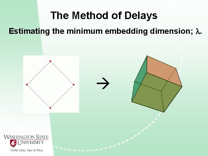
The Method of Delays Estimating the minimum embedding dimension; . • Kennel and Brown (PR: A 1992) developed the False Nearest Neighbors. • The False Nearest Neighbors technique uses Euclidean distances to determine if the vectors of Y are still “close” as the dimension of the phase space is increased.

The Method of Delays Estimating the minimum embedding dimension; .

Simulation • The simulation follows that in Chon et al (1997). • The Ikeda Map is numerically generated and the deterministic variable Xt is isolated. Ikeda Map

Simulation • • Six variables are constructed by adding contamination, i, t to the deterministic component, Xt, post numerical iteration. Z 1 is entirely deterministic and Z 6 is entirely random.

Simulation: Zi(t) Traditional tests of dependence confirm the presence of a process in Z 1 -Z 4.

Simulation Which one is deterministically generated, Z 1, and which one is randomly generated, Z 6?

Simulation: Z 1(t) = Xn + n, 1~N(0, 0) The structure of the process is well defined and appears to follow a stable trajectory.

Simulation: Z 3(t) = Xn + n, 3~N(0, 0. 125) • The contamination has a variance roughly equal to 25% of the deterministic process. • While the general direction of the trajectory paths remain; the tightness, or clarity, of the paths has greatly diminished.

Simulation: Z 5(t) = Xn + n, 5~N(0, 0. 5) • • • The phase portrait is close to that of Gaussian randomly generated data. Traditional methods of determining independence can no longer detect suspect behavior. The volatility of the contamination has overcome the deterministic component.

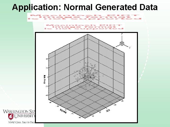
Simulation: Z 6(t) = n, 6~N(0, 0. 5) • The “ball” of a normal distribution is the benchmark for comparison and detection of nonlinear processes in regression residuals.

Simulation Which one is deterministically generated, Z 1, and which one is randomly generated, Z 6? Z 6, Randomly Generated Z 1, Deterministically Generated

ARMA Fitted Z 1(t) Residuals such as Z 1 will only appear in the presence of a nonlinear process and cannot be controlled for using linear techniques.

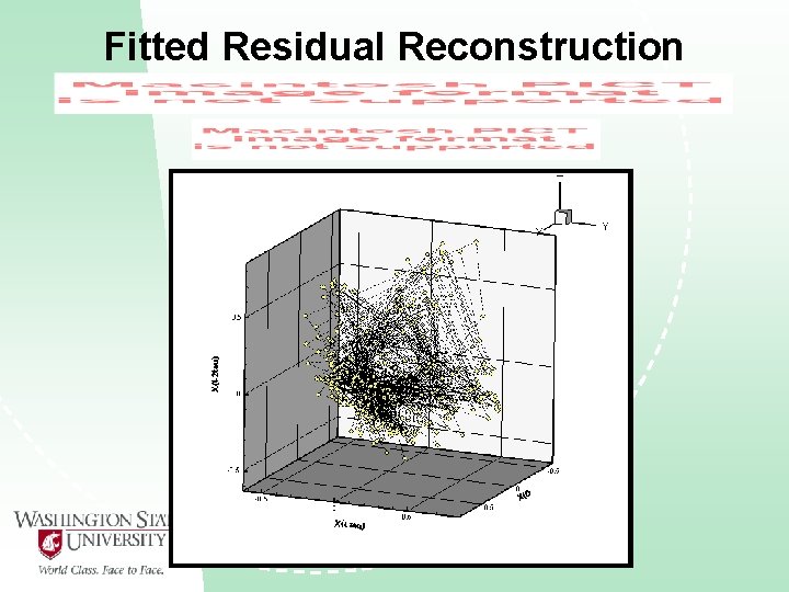
Fitted Residual Reconstruction

Insights from Simulations • If the first four time series of the simulation happened to be the residuals of an econometric model, model misspecification may have been concluded. • Having that qualitative representation of the residual structure in the phase space reconstruction may enhance additional modeling. • After the variance of the additive contamination increased above 25% of the variance of the deterministic component only general structure could be inferred. • After the variance of the contamination increased passed 50% of the deterministic component the ability to distinguish structure from noise decreased rapidly.

Application: The S&P 500 • Following Granger, Maasoumi, and Racine (JTSA 2004), regression residuals from a nonlinear time series model of S&P 500 from Jan. 3, 1996 to Dec. 22, 1997 are analyzed • A simple ARIMA model is fit first: • After inspection, however, the linear model does not fully capture all variability.

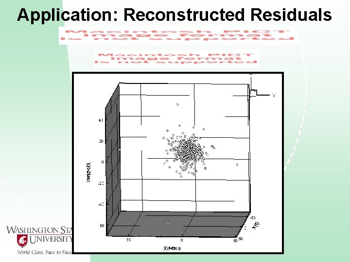
Application: Reconstructed Residuals

Application: The S&P 500 • An Integrated Auto Regressive Model with ARCH and GARCH structured residuals is fit to account for the discovered dependence.

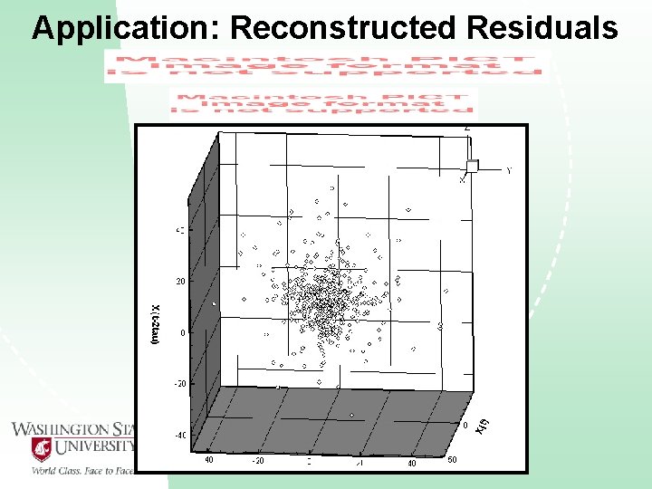
Application: Reconstructed Residuals

Application: Normal Generated Data

Final Observations • Given the similarity to random noise, we can find no strong visual evidence of nonlinear structure. • In cases when it is not sufficient to just detect dependence, phase space reconstruction can add valuable insight on the nature of the dependence. • Indeed, phase space reconstruction can be thought of as a nonlinear scatter plot. • The phase portrait may be used as a foundation for future model enhancement.

Questions?

Table 3: The average mutual information function for S&P 500 residual series.

Table 4: The percentage of false nearest neighbors for the S&P 500 residual series.