Superconducting electronics from Josephson effects to quantum computing


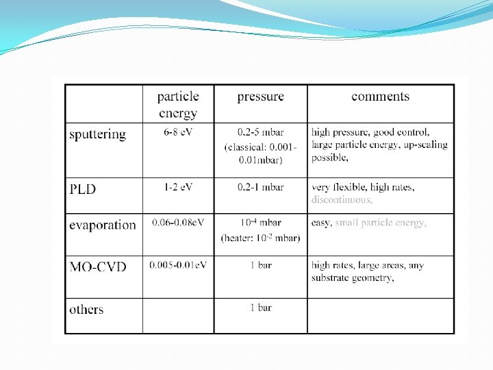
![Thin film preparation methods [R. Wördenweber]](https://slidetodoc.com/presentation_image_h2/81def57c997796372a709fb5fc171f16/image-4.jpg "Thin film preparation methods [R. Wördenweber]")


![Serial arrays for voltage standard [wikipedia]](https://slidetodoc.com/presentation_image_h2/81def57c997796372a709fb5fc171f16/image-8.jpg "Serial arrays for voltage standard [wikipedia]")
![[ J. Niemeier ] 9](https://slidetodoc.com/presentation_image_h2/81def57c997796372a709fb5fc171f16/image-9.jpg "[ J. Niemeier ] 9")
ROS-SQUID �Digital SQUIDs �Π-SQUID �Supercond. Quantum interference")
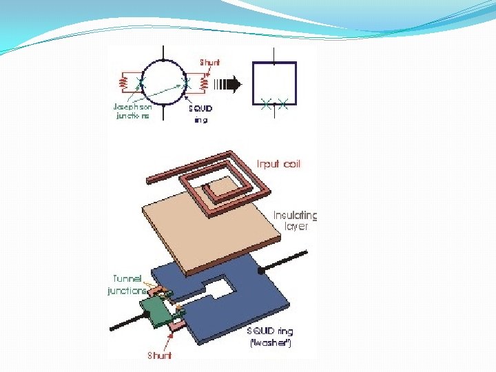
![[Gallop]](https://slidetodoc.com/presentation_image_h2/81def57c997796372a709fb5fc171f16/image-11.jpg "[Gallop]")


![LIC = 1. 25 Φ 0 k = 0 ↔ k =1 [Ruggiero, Rudman]](https://slidetodoc.com/presentation_image_h2/81def57c997796372a709fb5fc171f16/image-15.jpg "LIC = 1. 25 Φ 0 k = 0 ↔ k =1 [Ruggiero, Rudman]")
 Q = RT/ωrf LT M = K (LLT)½")


")

![Parameter [SQUID Handbook]](https://slidetodoc.com/presentation_image_h2/81def57c997796372a709fb5fc171f16/image-21.jpg "Parameter [SQUID Handbook]")
SQUIDs")
![Transition to films [SQUID Handbook]](https://slidetodoc.com/presentation_image_h2/81def57c997796372a709fb5fc171f16/image-23.jpg "Transition to films [SQUID Handbook]")

![HTS-RF-SQUID [FZ Jülich]](https://slidetodoc.com/presentation_image_h2/81def57c997796372a709fb5fc171f16/image-25.jpg "HTS-RF-SQUID [FZ Jülich]")


 for Ic 1 = Ic 2 = Ic (symmetrical) � Flux is")
 Approximation without flux contribution of the ring current ( this current is")


 Φ 0, n = 0, ±")

")


")

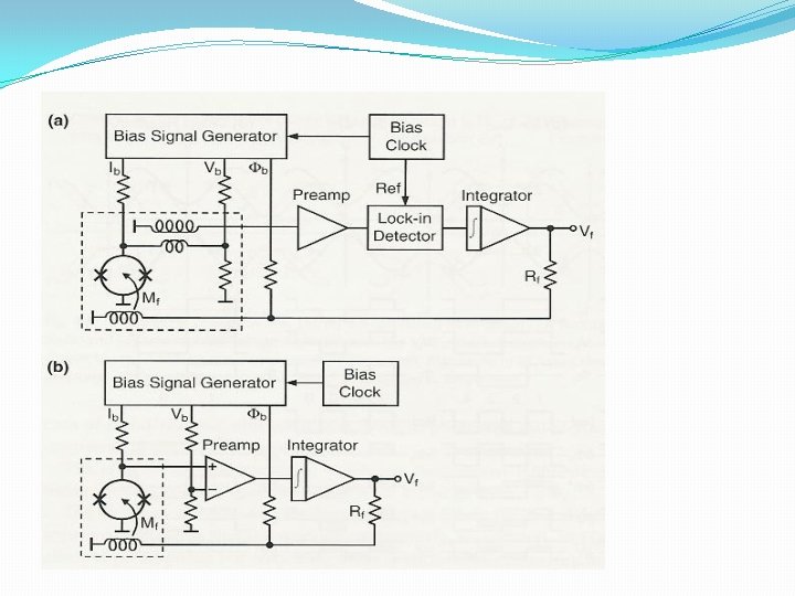
![[Drung]](https://slidetodoc.com/presentation_image_h2/81def57c997796372a709fb5fc171f16/image-47.jpg "[Drung]")
![Direct electronics with AFP (additional positive feedback) [Drung]](https://slidetodoc.com/presentation_image_h2/81def57c997796372a709fb5fc171f16/image-48.jpg "Direct electronics with AFP (additional positive feedback) [Drung]")


![Wire incoupling structures [ J. Clarke ]](https://slidetodoc.com/presentation_image_h2/81def57c997796372a709fb5fc171f16/image-52.jpg "Wire incoupling structures [ J. Clarke ]")
![Multi channel gradiometer [ Biomagnetisches Zentrum der FSU Jena ]](https://slidetodoc.com/presentation_image_h2/81def57c997796372a709fb5fc171f16/image-53.jpg "Multi channel gradiometer [ Biomagnetisches Zentrum der FSU Jena ]")


 FSU Jena 1984 Nb-Pb thin film technology")


![[Chesca]](https://slidetodoc.com/presentation_image_h2/81def57c997796372a709fb5fc171f16/image-68.jpg "[Chesca]")


 30 JJ SQIF and a simple SQUID of same size")
![Serial SQIF [Schultze]](https://slidetodoc.com/presentation_image_h2/81def57c997796372a709fb5fc171f16/image-74.jpg "Serial SQIF [Schultze]")
![2 p. T / √ Hz [IPHT Jena]}](https://slidetodoc.com/presentation_image_h2/81def57c997796372a709fb5fc171f16/image-75.jpg "2 p. T / √ Hz [IPHT Jena]}")
![2 D- SQIF array [R. Fagaly]](https://slidetodoc.com/presentation_image_h2/81def57c997796372a709fb5fc171f16/image-76.jpg "2 D- SQIF array [R. Fagaly]")
![Bi-SQUID [R. Fagaly]](https://slidetodoc.com/presentation_image_h2/81def57c997796372a709fb5fc171f16/image-77.jpg "Bi-SQUID [R. Fagaly]")
- Slides: 77
Superconducting electronics -from Josephson effects to quantum computing -by Pascal Febvre and Paul Seidel
Superconducting electronics – Part 2 Josephson junctions, arrays and SQUIDs
Josephson devices � Mainly thin film technology � Different types (SIS, SNS, SINIS, SFS, …) � Josephson � Complex junctions as active devices (e. g. mixers) superconducting circuits (e. g. RSFQ) � Different sensors (SQUIDs, SQUIFs, radiation detectors) 3
Thin film preparation methods [R. Wördenweber]
Patterning of films by lithography and etching
Arrays of Josephson junctions
Serial arrays for voltage standard [wikipedia]
[ J. Niemeier ] 9
SQUIDs Superconducting quantum interference devices �RF-SQUID �DC-SQUID �(D)ROS-SQUID �Digital SQUIDs �Π-SQUID �Supercond. Quantum interference filter (SQIF)
[Gallop]
RF-SQUID �non-linear inductance of Josephson junction gives a periodic modulation of the resonance frequency of the tank circuit �these changes follow the amplitude of the rf current for a given working frequency �response variies with Φ 0 = h/2 e = 2, 07 10 -15 Vs �advantage: no electrical contacts �disadvantage: noise of tank curcuit and amplifier large than intrinsic SQUID noise
RF-SQUID �Total flux Φ = Φex + LIC sin φ �Phase φ = 2 π Φ / Φ 0 �Φ = Φex + LIC sin (2 π Φ / Φ 0 ) �SQUID-Parameter ßrf = 2 π LIC / Φ 0
Characteristic of r. f. SQUID ßrf =0. 6 ßrf > 1
LIC = 1. 25 Φ 0 k = 0 ↔ k =1 [Ruggiero, Rudman]
Voltage of tank circuit (without noise) Q = RT/ωrf LT M = K (LLT)½ ωrf 20 MHz … 1 GHz Transfer function V Φ = ωrf LT / M
Transfer function �K can not be choosen too small ! �Irf has to cut the step for all flux values �for LIC ≈ Φ 0 follows K 2 Q ≥ π / 4 (≈ 1) �with K ≈ Q -1/2 results
With thermal noise
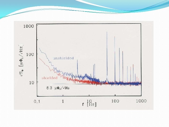
Noise of RF-SQUIDs �Intrinsic flux noise �Final step slope (thermal noise)
Energy resolution �Amplifier at room temperature and capacitive contributions of current lines result in an effective noise temperature
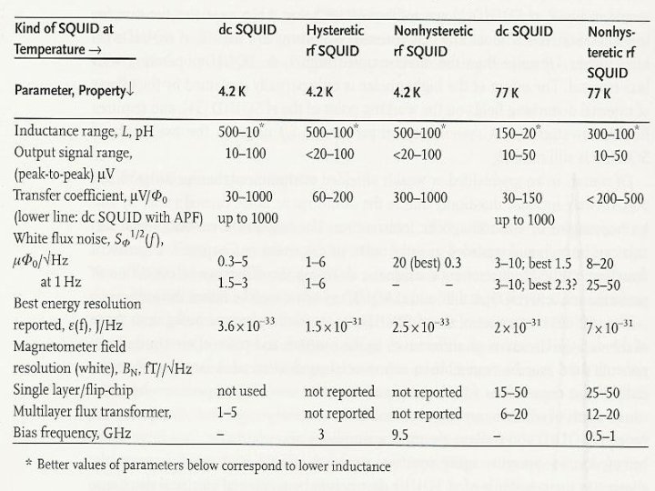
Parameter [SQUID Handbook]
Bulk (Zimmermann)SQUIDs
Transition to films [SQUID Handbook]
Zimmermann-SQUID IPTT Tschernogolovka/ FSU Jena about 1970 Niobium bulk Zimmermann-SQUID IPTM Tschernogolovka about 1975 Thin film –bulk hybrid technique [Meyer]
HTS-RF-SQUID [FZ Jülich]
Step-edge junction
HTS-RF-SQUID Resonator
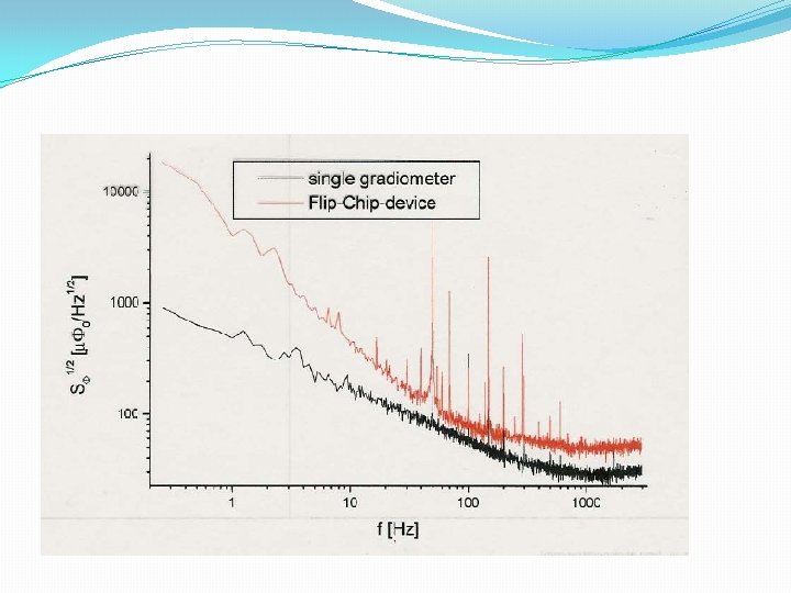
Comparison of noise
Noise characteristics
Planar microwave SQUID
DC-SQUID
Interference of the ring currents �Current splitting �Ring current J → I = I 1 + I 2 I 1 = +J I 2 = � Josephson currents I 1 = Icsinφ1 I 2 = Icsinφ2 -J
1. ) for Ic 1 = Ic 2 = Ic (symmetrical) � Flux is external Flux plus self field by ring current Φ = Φex + LJ � Phase difference is 2π-periodical φ2 – φ1 = 2 π Φ / Φ 0 = 2 π (Φex + LJ) / Φ 0
2. ) Approximation without flux contribution of the ring current ( this current is in general J < Ic thus LJ < LIc → should be << Φ 0 /2, i. e. << 1 Inductance (Ring) Parameter
With this assumption it is Φ = Φex and thus follows I = Ic [sinφ1 + sin (φ1 + 2πΦex/Φ 0)] with δ = φ1 + π Φex/Φ 0 and simple transformatios for sin functions results in I = 2 Ic sinδ cos (πΦex /Φ 0)
SQUID Modulation
Integer values of flux Φex = n · Φ 0 cos = 1 Maximum value Is, max = 2 Ic obtained Ring current disappears (sinφ1 = sinφ2 = 1)
Half integer values of flux �Φex = (n+1/2) Φ 0, n = 0, ± 1, ± 2, … �Is, max = 0 �Ring current reaches maximum (± Ic)
DC-SQUID Modulation
Asymmetric case �Is, max = Ic 1 + Ic 2 �but Is, max (Φ) nearer to the maximum �Modulation amplitude becomes smaller �Dependence on βL �optimum βL~ 1 (Limit for Aeff at fixed L)
Inductance parameter ßL ßL = 2 LIC / Φ 0
Influence of asymmetry
SQUID and junction modulation
Energy resolution
FFL-Electronics (flux locked loop)
Flux modulation
[Drung]
Direct electronics with AFP (additional positive feedback) [Drung]
bias reversal
Gradiometer types
Wire incoupling structures [ J. Clarke ]
Multi channel gradiometer [ Biomagnetisches Zentrum der FSU Jena ]
LTS-SQUIDs
The Jena SQUID UJ 111
UJ 111 (with lead shield) FSU Jena 1984 Nb-Pb thin film technology
Niobium 8 layers YBCO 1 layer Grain boundary
Planar DC-SQUID Gradiometer Superconducting antenna I 2 FSQ I 1 -I 2 B 1 B 2 Magnetic flux within SQUID
F. Schmidl, A. Zakasarenko, E. Il`ichev, P. Seidel
HTS DC-SQUID Gradiometer
Flux transformer
Pi-SQUIDs
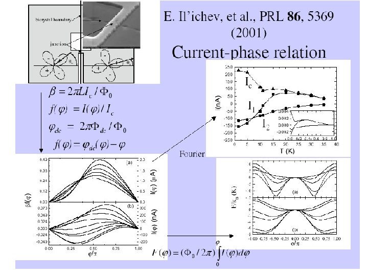
[Chesca]
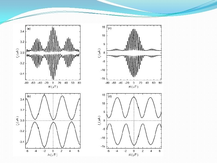
Comparison
Relaxation Oszillation SQUIDs
Digital SQUIDs
Quantum interference filter (SQIF) 30 JJ SQIF and a simple SQUID of same size [Oppenländer, Schopohl]
Serial SQIF [Schultze]
2 p. T / √ Hz [IPHT Jena]}
2 D- SQIF array [R. Fagaly]
Bi-SQUID [R. Fagaly]