The Argument Against Quantum Computers Gil Kalai IDC

The Argument Against Quantum Computers Gil Kalai IDC, Herzeliya; Yale University and The Hebrew University of Jerusalem IDC Herzli CERN Colloquium August 2019

CERN

SESAME An amazing scientific partnership between Jordan, Cyprus, Egypt, Iran, Israel, Pakistan, the Palestinian Authority, and Turkey SESAME (Synchrotron-light for Experimental Science and Applications in the Middle East) is a “thirdgeneration” synchrotron light source that was officially opened in Allan (Jordan) on 16 May 2017.

The mathematical theory of Noise sensitivity and stability

Outline: Nine models, four theorems, one conjecture Main puzzle: Are quantum computers possible? I will discuss the sensitivity of noisy intermediate scale quantum (NISQ) systems and provide an argument for why quantum computers are not possible. Related puzzle: The effect of errors in counting votes in elections. Our analysis is based on a theory of noise stability and noise sensitivity of voting rules and other processes. .

The argument against Quantum Computers Noisy intermediate scale quantum systems (NISQ systems) represent a low-level computational ability that will not allow using them for building quantum error-correcting codes that are needed for quantum computation. We need to explain why it is the case that error-correcting codes are needed for getting computational supremacy via quantum computing, and we also need to explain why quantum error correcting codes are out of reach.

In a few years we will know better

Part I: Computation Model 1: Boolean functions are functions f(x 1, x 2, …, xn) of n Boolean variables (xi=1 or xi=-1) so that the value of f is also -1 or 1. Boolean functions are of importance in combinatorics, probability theory, computer science, voting, and other areas. Examples. Majority: n is odd, f=1 if x 1+x 2+…+xn > 0. Dictatorship: f=x 1.

Model 2: Computers! (Boolean circuits) The basic memory component in classical computing is a bit, which can be in two states, “ 0” or “ 1”. A computer (or circuit) has �� bits, and it can perform certain logical operations on them. The NOT gate, acting on a single bit, and the AND gate, acting on two bits, suffice for the full power of classical computing.

Model 3: Polynomial size Boolean circuits A circuit with n input bits of size at most Anc. Here A and c are positive constants. Output: a single bit. Polynomial-size circuit (polynomial time computation, efficient computation)

Model 4 – Randomized circuits A circuit with n bits of input and with one additional type of gate that provides a random bit. Again we assume that the circuit is of size at most Anc (here, again, A and c are positive constants). This time the output is a sample from a probability distribution on strings of length k of zeroes and ones.

Efficient computation and Computational complexity • The complexity class P refers to problems that can be solved using a polynomial number of steps in the size of the input. • The complexity class NP refers to problems whose solution can be verified in polynomial number of steps. • Our understanding of the computational complexity world depends on a whole array of conjectures: NP ≠ P is the most famous one.

Model 5: Quantum computers Qubits are unit vectors in C 2: A qubit is a piece of quantum memory. The state of a qubit is a unit vector in a 2 -dimensional complex Hilbert space H = . The memory of a quantum computer (quantum circuit) consists of n qubits and the state of the computer is a unit vector in . Gates are unitary transformations: We can put one or two qubits through gates representing unitary transformations acting on the corresponding two- or four-dimensional Hilbert spaces, and as for classical computers, there is a small list of gates sufficient for the full power of quantum computing. Measurement: Measuring the state of k qubits leads to a probability distribution on 0– 1 vectors of length k.

Shor’s factoring theorem Theorem 1 (Peter Shor 1994): Quantum computers can factor �� -digit integers efficiently 2 steps! — in ∼ ��

Efficient computation and Computational complexity

Noisy quantum circuits Quantum systems are inherently noisy; we cannot accurately control them, and we cannot accurately describe them. In fact, every interaction of a quantum system with the outside world accounts for noise. Model 6: Noisy quantum circuits A quantum circuit such that every qubit is corrupted in every “computer cycle” with a small probability t, and every gate is timperfect. Here, t is a small constant called the rate of noise.

The Threshold Theorem 2: If the error rate is small enough, noisy quantum circuits allows the full power of quantum computing. Aharonov, Ben-Or (1995), Kitaev (1995), Knill, Lafflamme, Zurek (1995), following Shor (1995, 1995).

NISQ- circuits Model 7 – Noisy intermediate-scale quantum (NISQ) computers: These are simply noisy quantum circuits with at most 500 qubits.

NISQ devices - near term tasks Goal 1: Demonstrate quantum supremacy via systems of non-interacting bosons. (Baby goal 1 - ten bosons ) Goal 2: Demonstrate quantum supremacy on random circuits (namely, circuits that are based on randomly choosing the computation process, in advance), with 50 – 100 qubits. (Baby goal 2 – 10 -30 qubits ) Goal 3: Create distance-5 surface codes on NISQ circuits that require a little over 100 qubits. (Baby goal 3 - distance 3 surface code )

Part II: The argument against quantum computers. (A) Probability distributions described (robustly) by NISQ devices can be described by law-degree polynomials (LDP). LDP-distributions represent a very low-level computational complexity class well inside (classical) AC 0. (B) In the NISQ regime, asymptotically-low-level computational devices cannot lead to superior computation. (C) Achieving quantum supremacy is easier than achieving quantum error correction; quantum error correction is not supported by LDP. Therefore NISQ circuits do not support quantum error correction. There is strong theoretical evidence for (A) and empirical and theoretical evidence for (C).

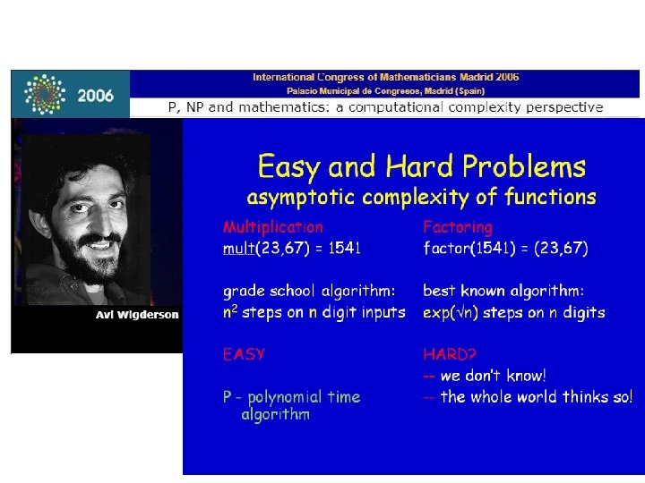
Permanents, determinants, and noise sensitivity of boson sampling • Multiplication is easy Factoring is hard! • Determinants are easy and Permanents are hard! Both these insights are very old. They were studied by mathematicians well before modern computational complexity was developed. Quantum computers make factoring easy, and also make computing permanents “easier”.

Boson sampling – the C. Elegans of quantum computing C. Elegans (Caenorhabditis elegans) is a species of a free-living roundworm whose biological study shed much light on more complicated organisms. Our next model, boson sampling can be seen as the C. elegans of quantum computing. It is both technically and conceptually simpler than the circuit model and yet it allows definite and clear-cut insights that extend to more general models and more complicated situations.

Model 8: Boson Sampling (non interacting bosons) Troyansky-Tishby (1996), Aaronson-Arkhipov (2010, 2013): Given a complex n by m matrix X with orthonormal rows. Sample subsets of columns (with repetitions) according to the absolute value-squared of permanents. This task is referred to as Boson Sampling. Quantum computers can perform Boson Sampling on the nose. There is a good theoretical argument by Aaronson. Arkhipov (2010) that these tasks are beyond reach for classical computers.

1 2 Input matrix Boson Sampling (permanents): {1, 1} – 0 {1, 2} – 1/6 {1, 3} – 1/6 {2, 2} – 2/6 {2, 3} – 0 {3, 3} – 2/6 Fermion Sampling (determinants): {1, 2} – 1/6 {1, 3} – 1/6 {2, 3} – 4/6 3

Model 9: Noisy Boson Sampling (Kalai-Kindler 2014) Let G be a complex Gaussian n x m noise matrix (normalized so that the expected row norms is 1). Given an input matrix A, we average the Boson Sampling distributions over (1 -t)1/2 A + t 1/2 G. t is the rate of noise. Now, expand the outcomes in terms of Hermite polynomials. The effect of the noise is exponential decay in terms of Hermite degree. The Hermite expansion for the Boson Sampling model is beautiful and very simple!

Noise stability/sensitivity of Boson. Sampling Theorem 3 (Kalai-Kindler, 2014): When the noise level is constant, distributions given by noisy Boson Sampling are well approximated by their low-degree Fourier-Hermite expansion. (Consequently, these distributions can be approximated by bounded-depth polynomial-size circuits. ) Theorem 4 (Kalai-Kindler, 2014): When the noise level is larger than 1/�� noisy boson sampling are very sensitive to noise, with a vanishing correlation between the noisy distribution and the ideal distribution.

The huge computational gap (left) between Boson Sampling (purple) and Fermion Sampling (green) vanishes in the noisy version.

From boson sampling to NISQ systems Conjecture 1: Both 2014 theorems of Kalai and Kindler extend to all NISQ systems (in particular, to noisy quantum circuits) and to all realistic forms of noise. (A) Probability distributions described (robustly) by NISQ devices can be described by law-degree polynomials (LDP). From the point of view of computational complexity, NISQ systems are primitive classical computational devices!

Predictions of near-term experiments Based on Theorems 3 and 4 and conjecture 1 For the distribution of 0 -1 strings based on a quantum pseudorandom circuit, or a circuits for surface code: a) For a larger amount of noise- you can get robust experimental outcomes but they will represent LDP (Low Degree Polynomials)- distributions which are far-away from the desired noiseless distributions. b) For a wide range of a smaller amount of noise- your outcome will be chaotic. This means that the resulting distribution will strongly depend on fine properties of the noise and that you will not be able to reach robust experimental outcomes at all.

(A) The computational power of NISQ systems NISQ-circuits are computationally very weak, unlikely to allow quantum codes needed for quantum computers.

The argument against quantum computers (B) (A) Probability distributions described (robustly) by NISQ devices can be described by law-degree polynomials (LDP). LDP-distributions represent a very low-level computational complexity class well inside (classical) AC 0. (B) In the NISQ regime, asymptotically-low-level computational devices cannot lead to superior computation. (C) Achieving quantum supremacy is easier than achieving quantum error correction; quantum error correction is not supported by LDP. Therefore NISQ circuits do not support quantum error correction.

Can physics make hard computations easy: Aaronson’s Soap Bubble Computer Physical devices cannot be engineered to solve NP-complete problems Noisy intermediate scale quantum (NISQ) circuits are computationally much more primitive than soap bubble computers and this will prevent them from achieving neither "quantum supremacy" nor good quality quantum error correcting codes.

The crux of the debate I argue that from the point of view of computational complexity NISQ devices are, in fact, low-level classical computing devices, and I regard it as strong evidence that engineers will not be able to reach the level of noise required for quantum supremacy. Others argue that the existence of low-level simulation (in the NISQ regime) for every fixed level of noise does not have any bearing on the engineering question of reducing the level of noise. These sharply different views will be tested in the next few years.

Part III: The failure of quantum computers - Underlying principles and consequences

Consequences for cats Following the tradition of using cats for quantum thought experiments, consider an ordinary living cat. If quantum computation is not possible, • It will be impossible to teleport the cat; • It will be impossible to reverse time in the life of the cat; • It will be impossible to implement the cat on a very different geometry; • it will be impossible to superpose the lives of two distinct cats; • the life of this cat cannot be predicted. Here, our “cat” may represent realistic (but involved) quantum evolutions described by quantum circuits with less than 50 qubits. Baby goals 1– 3 can serve as good candidates for such “cats. ”

Lewis Wein (look him up)

Noise stability and sensitivity for models of HEP? An interesting direction for future research would be to extend the mathematical noise stability/noise sensitivity dichotomy and to find relevant Fourier-like expansions and definitions of noise for mathematical objects of high-energy physics. In particular, to models where the groups Z/2 Z or S 1 are replaced by other groups relevant to physics (e. g. SU(2), SU(3)). And to find more examples for noise stability.

Conclusion Integrating computational modeling, algorithms, and complexity into theories of nature and society, marks a new scientific revolution! Avi Wigderson, Mathematics and Computation, Princeton 2019. Understanding noisy quantum systems and potentially even the failure of quantum computers is related to the fascinating mathematics of noise stability and noise sensitivity and its connections to theory of computing. Exploring this avenue may have important implications to various areas of quantum physics.

Thank you very much! ! תודה רבה

Important analogies • The analogy between classical and quantum computers • The analogy between quantum circuits and Boson. Sampling • The analogy between different realizations of quantum computers: via superconducting qubits, via trapped atomic ions, via photons, … • The analogy between surface codes that Google tries to build and topological quantum computing pursued by Microsoft • The analogy between Majorana fermions in high energy physics and in condensed matter physics.