Online learning and game theory Adam Kalai joint

Online learning and game theory Adam Kalai (joint with Sham Kakade)

How do we learn? n n Goal learn a function f: X ! Y Batch (offline) model q =? q n Y = {–, +} Get training data (x 1, y 1), …, (xn, yn) drawn independently from some distribution over X £ Y We output f: X ! Y with low error P [f(x) y] Online (repeated game) model, for i=1, 2, …, n: q q Observe ith example xi 2 X Distribution-free We predict its label learning Observe true label yi 2 {–, +} Goal: make as few mistakes as possible

Outline 1. Online/batch learnability of F q q q 2. Online learnability ) batch learnability Finite learning: batch and online (via weighted maj. ) Batch learnability , online learnability? Online learning in repeated games q q Zero-sum: Weighted majority General-sum: No “internal regret” ) corr. eq.

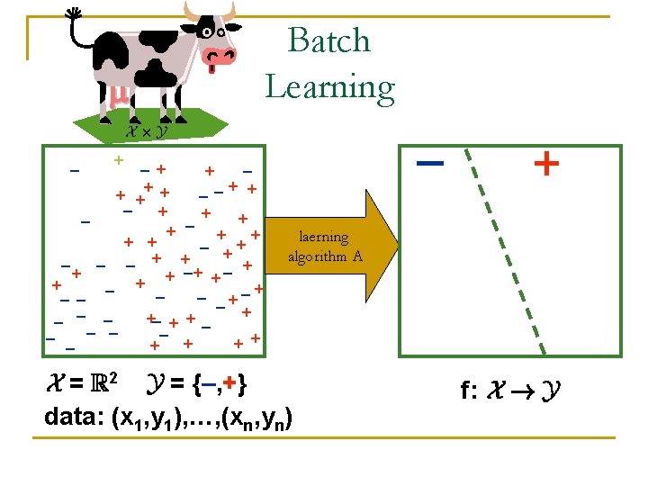
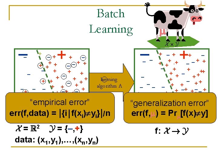
Online learning “empirical error” err(A, data) = |{i j zi yi}|/n n – n – … ? n + n n X = R 2 Y = {–, +} Online alg. A(x 1, y 1, …, xi-1, yi-1, xi)=zi n Adversary picks (x 1, y 1) 2 X £ Y We see x 1 We predict z 1 We see y 1 Adversary picks (xn, yn) 2 X £ Y We see xn We predict zn We see yn

Online/batch learnability of F n n Family F of functions f: X ! Y (Y = {–, +}) Alg. A learns F online if 9 k, c>0 q q Online input: data (x 1, y 1), …, (xn, yn) Regret(A, data) = err(A, data)–ming 2 F err(g, data) 8 data E[Regret(A, data)] · k/nc n Alg. B batch learns F if 9 k, c>0 q q X£Y Input: (x 1, y 1), …, (xn, yn) independent from Output: f 2 F, Regret(f, ) = err(f, )–ming 2 F err(g, ) 8 Edata[Regret(B, )] · k/nc

Online learnable ) Batch learnable n n Given online learning algorithm A Define batch learning algorithm B q q q n Input: (x 1, y 1), (x 2, y 2), …, (xn, yn) from Let fi(x): X ! Y be fi(x)=A(x 1, y 1, …, xi-1, yi-1, x) · Pick i 2 {1, 2, …, n} at random and output fi Analysis E[Regret(A, data)] = E[err(A, data)] – E[ming 2 F err(g, data)] E[Regret(B, )] = E[err(B, )] – ming 2 F err(g, )

Online learnable ) Batch learnable n Given online learning algorithm A Define batch learning algorithm B q q q n Input: (x 1, y 1), (x 2, y 2), …, (xn, yn) from Let fi(x): X ! Y be fi(x)=A(x 1, y 1, …, xi-1, yi-1, x) · Pick i 2 {1, 2, …, n} at random and output fi Analysis E[Regret(A, data)] = E[err(A, data)] – E[ming 2 F err(g, data)] · = · n E[Regret(B, )] = E[err(B, )] – ming 2 F err(g, )

Outline 1. Online/batch learnability of F ü q q q 2. Online learnability ) batch learnability Finite learning: batch and online (via weighted maj. ) Batch learnability ; online learnability ti uc ve Batch learnability )transd online learnability Online learning in repeated games q q Zero-sum: Weighted majority ) eq. General-sum: No “internal regret” ) corr. eq.

Online majority algorithm f 1 f 2 f 3 … f. F x 1 x 2 x 3 … xn + – – + + … …… + + – (live) majority + + + truth y + – – n n n Perfect f 2 F Say there is some perfect f* 2 F, err(f*, data)=0 Say |F|=F Predict according to majority of consistent f’s Each mistake Maj makes eliminates ¸ ½ of f’s Maj’s #mistakes · log 2(F) err(Maj, data) · log 2(F)/n

Naive batch learning f 1 f 2 f 3 … f. F x 1 x 2 x 3 … xn + – – – + + + – … …… … + + – – n n truth y + – – Perfect f 2 F Say there is some perfect f* 2 F, err(f*, data)=0 Say |F|=F Select a consistent f Say 8 g f* err(g, data)=log(F)/n – P[err(g, data)=0]= Wow! Online looks like batch.

Naive batch learning n Naive batch algorithm q Choose f 2 F that minimizes err(f, data) For any f 2 F, P[|err(f, data)-err(f, )|> P[9 f 2 F |err(f, data)-err(f, )|> ]· 2 -2 c 2 e ] · 2 Fe-200 ln F · 2 -100 E[Regret(n. b. , )] · c (F = |F|)

Weighted majority’ [LW 89] n Assign weight to each f, 8 f 2 F w(f)=1 n On period i=1, 2, …, n: q q Predict weighted maj of f’s For each f: if f(xi) yi, w(f): =w(f)/2 WM’ errs ) total weight decreases by ¸ 25% n Final total weight · F (3/4)#mistakes(WM’) n Final total weight ¸ 2 -minf #mistakes(f) #mistakes(WM’)· 2. 41(minf#mistakes(f)+log(F)/n) n (F = |F|)

Weighted majority [LW 89] n Assign weight to each f, 8 f 2 F w(f)=1 n On period i=1, 2, …, n: q q n Predict weighted maj of f’s For each f: if f(xi) yi, w(f): =w(f)(1– ) Thm: E[Regret(WM, data)] · 2 Wow! Online looks like batch. (F = |F|)

Weighted majority extensions… W n f 1 f 2 f 3 … f. F x 1 x 2 x 3 … xn + – – + + … …… + + – WM + + + truth y + – – Tracking q On any window W, E[Regret(WM, W)]· c

Weighted majority extensions… n f 1 f 2 f 3 … f. F x 1 x 2 x 3 … xn + – + … …… Multi-armed bandit q q WM + + + truth y – – – You don’t see xi You pick f Find out if you erred E[Regret] · c

Outline 1. Online/batch learnability of F ü q Finite learning: batch and online (via weighted maj. ) Batch learnability ; online learnability q Batch learnability ) (transductive) online learnability ü 2. Online learnability ) batch learnability Online learning in repeated games q q Zero-sum: Weighted majority ) eq. General-sum: No “internal regret” ) corr. eq.

Batch Online n n Define fc: [0, 1] ! {+, –}, fc(x) = sgn(x – c) Simple threshold functions F = {fc | c 2 [0, 1]} Batch learnable: Yes Online learnable: ? No! q q q Adversary does a “random binary search” Each label is equally likely to be +/– E[Regret]=½ for any online algorithm – – + 0 x 2 x 4 x 5 x 3 + x 1=. 5 1

Key idea: transductive online learning [Kakade. K 05] n n We see x 1, x 2, …, xn 2 X in advance y 1, y 2, …, yn 2 {+, –} are revealed online – – + 0 x 2 x 4 x 3 + x 1=. 5 1

Key idea: transductive online learning “empirical error” err(A, data) = |{i j zi yi}|/n [Kakade. K 05] n n – – n n ? n + n Adversary picks (x 1, y 1), …, (xn, yn)2 X£Y Adversary reveals x 1, x 2, …, xn We predict z 1 We see y 1 We predict z 2 We see y 2 … n X = R 2 Y = {–, +} n We predict zn We see yn Trans. online alg. T(x 1, y 1, …, xi-1, yi-1, xi+1, …, xn)=zi

Algorithm for trans. online learning [KK 05] n n n We see x 1, x 2, …, xn 2 X in advance y 1, y 2, …, yn 2 {+, –} are revealed online Algorithm for trans. online learning q q L distinct labelings f(x 1), f(x 2), …, f(xn) over all f 2 F Effective size of F is L Run WM on L functions E[Regret(WM, data)] · 2 f 1 f 2 f 3 … f 1 x 2 x 3 … xn + – + + + + + – … …… … + + – –

How many labelings? Shattering & VC n Def: S µ X is shattered if there are 2|S| ways to label S by f 2 F VC(F) = max|S| S is shattered by F n Example n – + – + n + + VC dimension captures complexity of F –

How many labelings? Shattering & VC n Sauer’s lemma: # labelings L = O(n. VC(F)) ) E[Regret(WM, data)] ·

Cannot batch learn faster than VC(F) Shattered set S, |S| = VC(F), n > 0 Batch training set of size n n Each x 2 S is not in training set with probability (1 -1/n)n ¼ e-1 ) E[Regret(B, )] ¸ c. VC(F)/n n X£Y

Putting it together n Transductive online: E[Regret(WM, data)] = n Batch: E[Regret(B, )] ¸ Almost identical to standard VC bound Trans. online learnable , batch learnable , finite VC(F)

Learnability conclusions n n n Finite VC(F) characterizes batch and transductive learnability Open problem: what propertyof F characterizes online learnability (nontransductive) Efficiency!? q q WM algorithm requires enumeration of F Thm [KK 05]: if one can efficiently find lowest error f 2 F, then one can design efficient online learning algorithm

Online learning in repeated games

Repeated games Pl. 2 R n Example: Pl. 1 R P S n 0, 0 P S -1, 1 1, -1 -1, 1 0, 0 Rounds i=1, 2, …, n: q q Players simultaneously choose actions Players receive payoff, goal: max total payoff Learning: players need not know opponent/game Feedback: player only finds out payoff of his action and alternatives (not opponent action)

(Mixed) Nash Equlibrium n n Each player chooses a dist. over actions Players are optimizing relative to opponent(s) 1/3 R P 1/3 S 1/3 1/3 R P S 0, 0 -1, 1 1, -1 -1, 1 0, 0

Online learning in 0 -sum games (Schapire recap) Payoff is A(i, j) for pl. 1, -A(i, j) for pl. 2 n Going first is disadvantage: maxi minj A(i, j) · minj maxi A(i, j) n Mixed strategies: n max min A( , ) · min max A( , ) n n Min-max theorem “=”

Online learning in 0 -sum games (Schapire recap) n Each player uses weighted majority q q q n n Maintain weight on each action, initially equal Choose an action proportional to weight (assume payoffs are in [-1, 1]) Find out payoffs of each action For each action weight à weight*(1 + payoff) Regret = possible improvement (in hindsight) from always playing a single action WM ) regret is low

Online learning in 0 -sum games (Schapire recap) n n n Actions are (a 1, b 1), (a 2, b 2), …, (an, bn) Regret of pl. 1 is Let be empirical distributions of actions a 1, …, an and b 1, …, bn, respectively =

Online learning in 0 -sum games (Schapire recap) WM ) “min-max” theorem max min A( , ) = min max A( , ) = “value of game” n Using WM, each player guarantees regret ! 0, regardless of opponent n q q q Can beat an idiot in tic-tac-toe Reasonable strategy to use Justifies how such equilibria might arise

General-sum games A A n n B 1, 1 0, 0 2, 2 No unique “value” B Many very different equilibria e. g. Can’t naively improve a “no regret” algorithm (by playing a single mixed strategy) Low regret for both players ; equilibrium

General sum games n Low regret ; Nash equilibrium, e. g. , (1, 1), (2, 2), … 1 2 3 4 1 2 0, 0 -1, -1 1, 1 -1, -1 0, 0 -1, 1 3 1, 1 1, -1 1, 1 4 1, -1 1, 1

Refined notion of regret n n Can’t naively improve a “no regret” algorithm (by playing a single mixed strategy) Might be able to naively improve it by replacing: “When alg. suggests 1, play 3” 1 2 3 4 1 2 0, 0 -1, -1 1, 1 -1, -1 0, 0 -1, 1 3 1, 1 1, -1 1, 1 4 1, -1 1, 1

Internal regret n n Internal regret IR(i, j) is how much we could have improved by replacing all occurrences of action i with action j No internal regret ) correlated equilibrium Calibration ) correlated equilibrium [Foster. Vohra] Correlated Equilibrium Play col. 2 [Aumann] 1, 0 0, 11/6 0, 0 1/6 q Best strategy to listen to the fish Play row 1 0, 0 1, 01/6 0, 11/6 0, 0 1, 01/6

Low internal regret ! correlated eq. n n n Sequence like (1, 1), (2, 1), (3, 2), … Think about this as a distribution P No internal regret , correlated eq. Play col. 2 1, 0 1/6 Play row 1 0, 11/6 0, 0 1, 01/6

Online learning in games conclusions n Online learning in zero-sum games q q n Online learning in general-sum games q q n Weighted majority (low regret) Achieves value of game Low internal regret Achieves correlated equilibrium Open problems q Are there natural dynamics ) Nash Equilibrium q Is correlated equilibrium going take over?