Online Learning of Quantum States Scott Aaronson UT

Online Learning of Quantum States Scott Aaronson (UT Austin) Joint work with Xinyi Chen, Elad Hazan, Satyen Kale, and Ashwin Nayak ar. Xiv: 1802. 09025 / Neur. IPS 2018

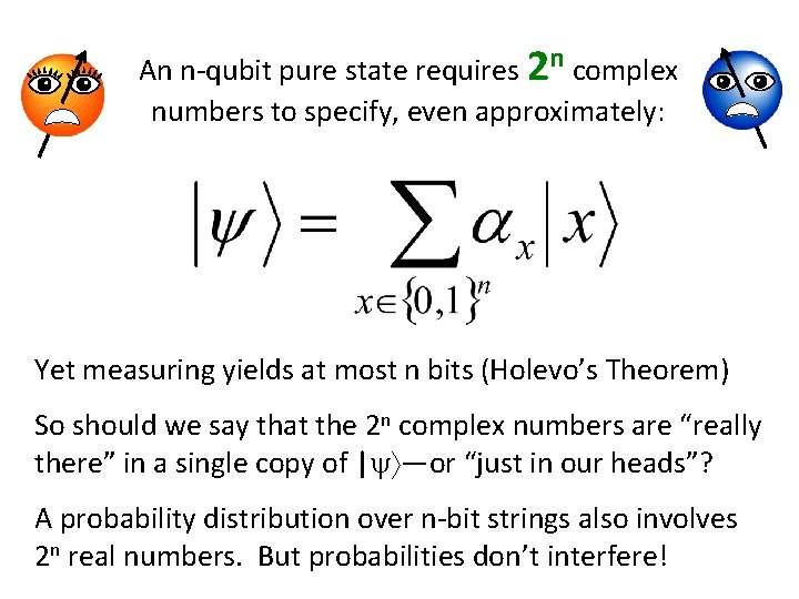
An n-qubit pure state requires 2 n complex numbers to specify, even approximately: Yet measuring yields at most n bits (Holevo’s Theorem) So should we say that the 2 n complex numbers are “really there” in a single copy of | —or “just in our heads”? A probability distribution over n-bit strings also involves 2 n real numbers. But probabilities don’t interfere!

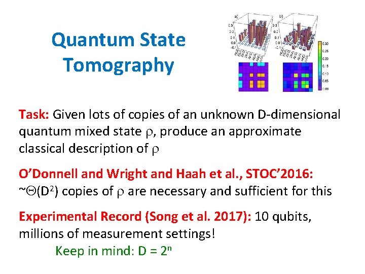
Quantum State Tomography Task: Given lots of copies of an unknown D-dimensional quantum mixed state , produce an approximate classical description of O’Donnell and Wright and Haah et al. , STOC’ 2016: ~ (D 2) copies of are necessary and sufficient for this Experimental Record (Song et al. 2017): 10 qubits, millions of measurement settings! Keep in mind: D = 2 n

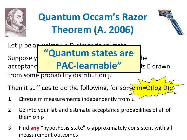
Quantum Occam’s Razor Theorem (A. 2006) Let be an unknown D-dimensional state “Quantum states are Suppose you just want to be able to estimate the acceptance probabilities of most measurements E drawn PAC-learnable” from some probability distribution Then it suffices to do the following, for some m=O(log D): 1. Choose m measurements independently from 2. Go into your lab and estimate acceptance probabilities of all of them on 3. Find any “hypothesis state” approximately consistent with all measurement outcomes

Can prove by combining two facts: (1) The class of [0, 1]-valued functions of the form f(E)=Tr(E ), where is a D-dimensional mixed state, has -fat-shattering dimension O((log D)/ 2) Largest k for which we can find inputs x 1, …, xk, and values a 1, …, ak [0, 1], such that all 2 k possible behaviors involving f(xi) exceeding ai by or vice versa are realized by some f in the class (2) Any class of [0, 1]-valued functions is PAC-learnable using a number of samples linear in its fat-shattering dimension [Alon et al. , Bartlett-Long]

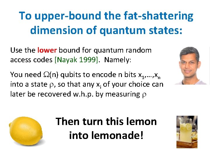
To upper-bound the fat-shattering dimension of quantum states: Use the lower bound for quantum random access codes [Nayak 1999]. Namely: You need (n) qubits to encode n bits x 1, …, xn into a state , so that any xi of your choice can later be recovered w. h. p. by measuring Then turn this lemon into lemonade!

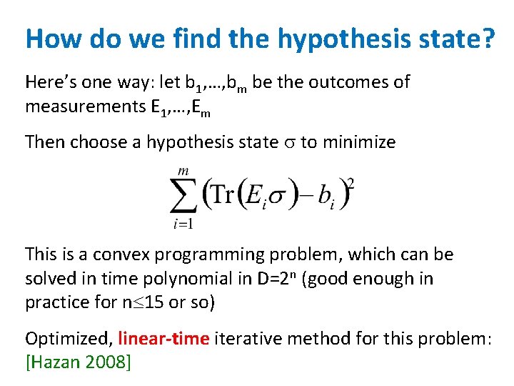
How do we find the hypothesis state? Here’s one way: let b 1, …, bm be the outcomes of measurements E 1, …, Em Then choose a hypothesis state to minimize This is a convex programming problem, which can be solved in time polynomial in D=2 n (good enough in practice for n 15 or so) Optimized, linear-time iterative method for this problem: [Hazan 2008]

You know, PAC-learning is so 1990 s. Who wants to assume a fixed, unchanging distribution over the sample data? These days all the cool kids prove theorems about online learning. What’s online learning?

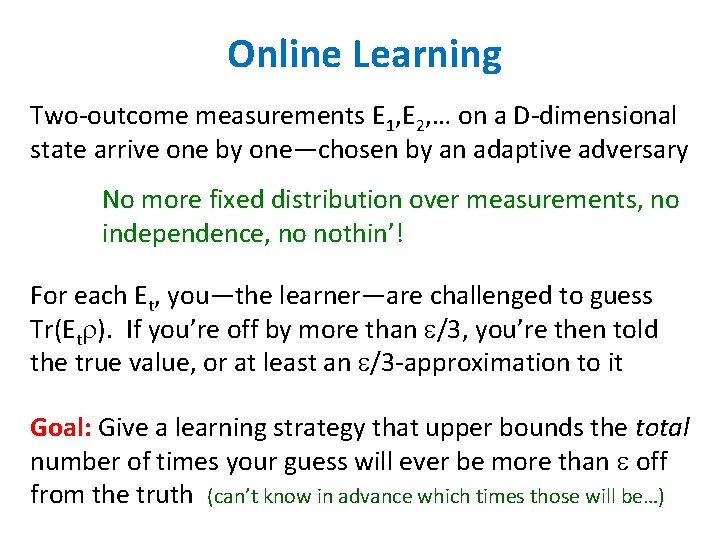
Online Learning Two-outcome measurements E 1, E 2, … on a D-dimensional state arrive one by one—chosen by an adaptive adversary No more fixed distribution over measurements, no independence, no nothin’! For each Et, you—the learner—are challenged to guess Tr(Et ). If you’re off by more than /3, you’re then told the true value, or at least an /3 -approximation to it Goal: Give a learning strategy that upper bounds the total number of times your guess will ever be more than off from the truth (can’t know in advance which times those will be…)

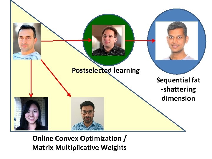
Postselected learning Sequential fat -shattering dimension Online Convex Optimization / Matrix Multiplicative Weights

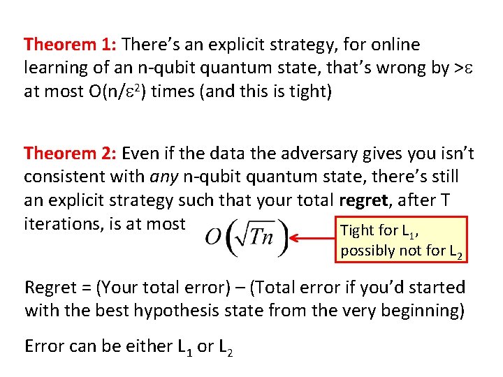
Theorem 1: There’s an explicit strategy, for online learning of an n-qubit quantum state, that’s wrong by > at most O(n/ 2) times (and this is tight) Theorem 2: Even if the data the adversary gives you isn’t consistent with any n-qubit quantum state, there’s still an explicit strategy such that your total regret, after T iterations, is at most Tight for L , 1 possibly not for L 2 Regret = (Your total error) – (Total error if you’d started with the best hypothesis state from the very beginning) Error can be either L 1 or L 2

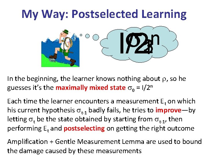
My Way: Postselected Learning n I/2132 In the beginning, the learner knows nothing about , so he guesses it’s the maximally mixed state 0 = I/2 n Each time the learner encounters a measurement Et on which his current hypothesis t-1 badly fails, he tries to improve—by letting t be the state obtained by starting from t-1, then performing Et and postselecting on getting the right outcome Amplification + Gentle Measurement Lemma are used to bound the damage caused by these measurements

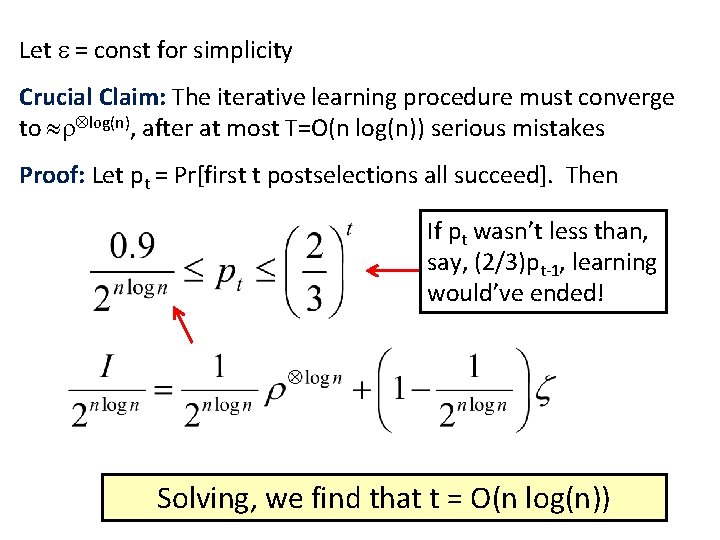
Let = const for simplicity Crucial Claim: The iterative learning procedure must converge to log(n), after at most T=O(n log(n)) serious mistakes Proof: Let pt = Pr[first t postselections all succeed]. Then If pt wasn’t less than, say, (2/3)pt-1, learning would’ve ended! Solving, we find that t = O(n log(n))

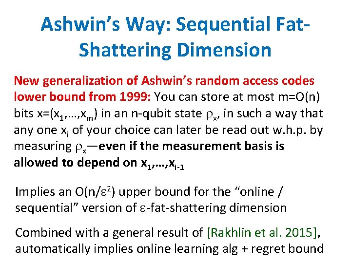
Ashwin’s Way: Sequential Fat. Shattering Dimension New generalization of Ashwin’s random access codes lower bound from 1999: You can store at most m=O(n) bits x=(x 1, …, xm) in an n-qubit state x, in such a way that any one xi of your choice can later be read out w. h. p. by measuring x—even if the measurement basis is allowed to depend on x 1, …, xi-1 Implies an O(n/ 2) upper bound for the “online / sequential” version of -fat-shattering dimension Combined with a general result of [Rakhlin et al. 2015], automatically implies online learning alg + regret bound

Elad, Xinyi, Satyen’s Way: Online Convex Optimization Regularized Follow-the-Leader [Hazan 2015] Gradient descent using von Neumann entropy Matrix Multiplicative Weights [Arora and Kale 2016] Technical work: Generalize power tools that already existed for real matrices to complex Hermitian ones Yields optimal mistake bound and regret bound

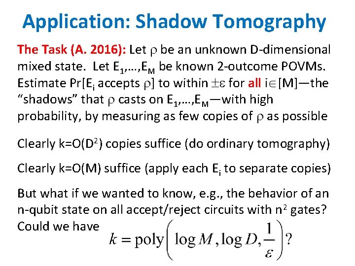
Application: Shadow Tomography The Task (A. 2016): Let be an unknown D-dimensional mixed state. Let E 1, …, EM be known 2 -outcome POVMs. Estimate Pr[Ei accepts ] to within for all i [M]—the “shadows” that casts on E 1, …, EM—with high probability, by measuring as few copies of as possible Clearly k=O(D 2) copies suffice (do ordinary tomography) Clearly k=O(M) suffice (apply each Ei to separate copies) But what if we wanted to know, e. g. , the behavior of an n-qubit state on all accept/reject circuits with n 2 gates? Could we have

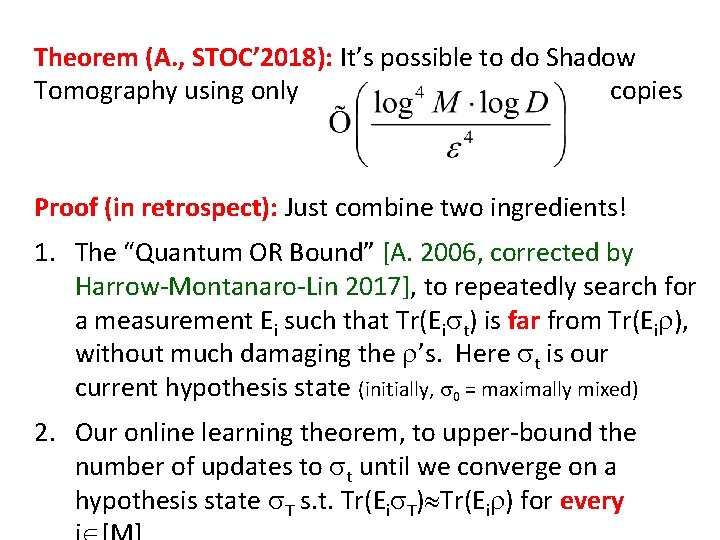
Theorem (A. , STOC’ 2018): It’s possible to do Shadow Tomography using only copies Proof (in retrospect): Just combine two ingredients! 1. The “Quantum OR Bound” [A. 2006, corrected by Harrow-Montanaro-Lin 2017], to repeatedly search for a measurement Ei such that Tr(Ei t) is far from Tr(Ei ), without much damaging the ’s. Here t is our current hypothesis state (initially, 0 = maximally mixed) 2. Our online learning theorem, to upper-bound the number of updates to t until we converge on a hypothesis state T s. t. Tr(Ei T) Tr(Ei ) for every

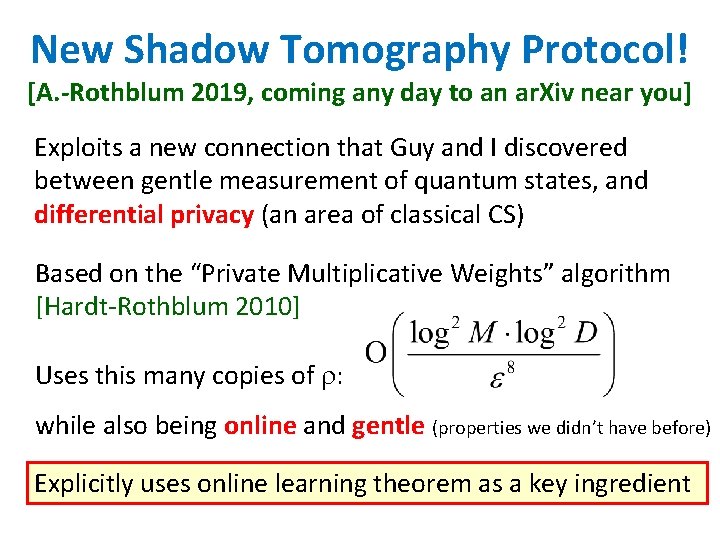
New Shadow Tomography Protocol! [A. -Rothblum 2019, coming any day to an ar. Xiv near you] Exploits a new connection that Guy and I discovered between gentle measurement of quantum states, and differential privacy (an area of classical CS) Based on the “Private Multiplicative Weights” algorithm [Hardt-Rothblum 2010] Uses this many copies of : while also being online and gentle (properties we didn’t have before) Explicitly uses online learning theorem as a key ingredient

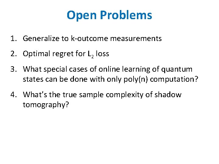
Open Problems 1. Generalize to k-outcome measurements 2. Optimal regret for L 2 loss 3. What special cases of online learning of quantum states can be done with only poly(n) computation? 4. What’s the true sample complexity of shadow tomography?