1 Shadow Tomography of Quantum States Scott Aaronson

1 Shadow Tomography of Quantum States Scott Aaronson (University of Texas at Austin) Technion, January 22, 2018

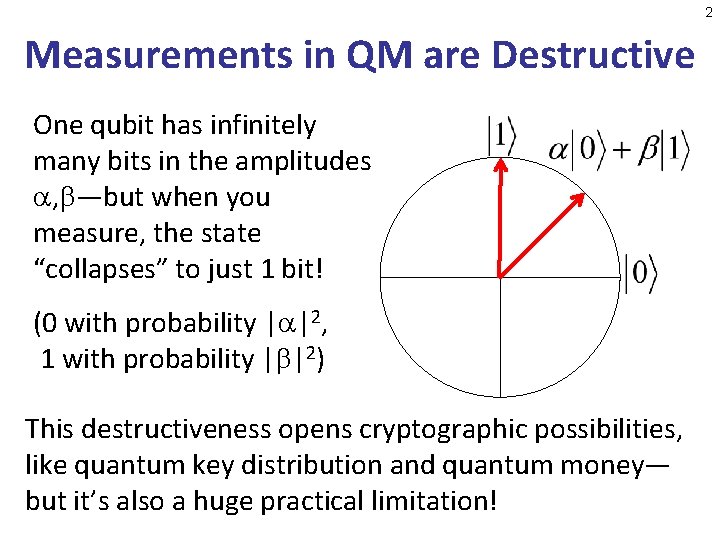
2 Measurements in QM are Destructive One qubit has infinitely many bits in the amplitudes , —but when you measure, the state “collapses” to just 1 bit! (0 with probability | |2, 1 with probability | |2) This destructiveness opens cryptographic possibilities, like quantum key distribution and quantum money— but it’s also a huge practical limitation!

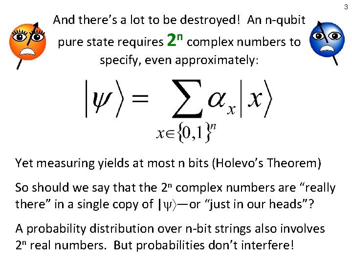
3 And there’s a lot to be destroyed! An n-qubit pure state requires 2 n complex numbers to specify, even approximately: Yet measuring yields at most n bits (Holevo’s Theorem) So should we say that the 2 n complex numbers are “really there” in a single copy of | —or “just in our heads”? A probability distribution over n-bit strings also involves 2 n real numbers. But probabilities don’t interfere!

4 Quick Review: Mixed States D D Hermitian positive semidefinite matrix with Tr( )=1 The most general kind of state in QM: encodes (everything measurable about) a distribution where each superposition | i occurs with probability pi A yes-or-no measurement can be represented by a D D Hermitian psd matrix E with all eigenvalues in [0, 1] The measurement “accepts” with probability Tr(E ), and “rejects” with probability 1 -Tr(E )

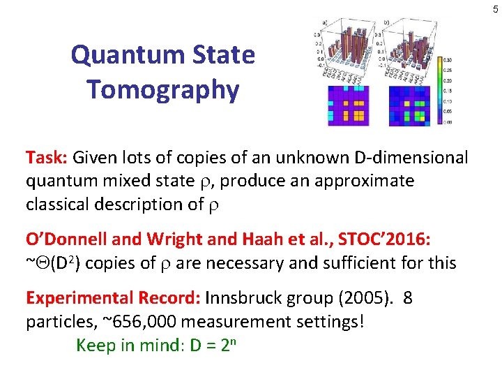
5 Quantum State Tomography Task: Given lots of copies of an unknown D-dimensional quantum mixed state , produce an approximate classical description of O’Donnell and Wright and Haah et al. , STOC’ 2016: ~ (D 2) copies of are necessary and sufficient for this Experimental Record: Innsbruck group (2005). 8 particles, ~656, 000 measurement settings! Keep in mind: D = 2 n

6 Quantum Computing Skepticism Levin Goldreich ‘t Hooft Davies Kalai Some physicists and computer scientists believe quantum computers will be impossible for a fundamental reason For many of them, the problem is that a quantum computer would “manipulate an exponential amount of information” using only polynomial resources But in what senses is it really an exponential amount?

7 Can we tame the exponential beast? Idea: “Shrink quantum states down to reasonable size” by asking what they’ll actually be used for In a sequence of works for 14 years, we’ve been using tools from computational learning theory to do exactly that: • Postselected learning theorem [A. 2004] • Quantum Occam’s Razor Theorem [A. 2006] • Full characterization of quantum advice [A. -Drucker 2010] • Shadow tomography theorem [A. 2017] • Online learning of quantum states [A. -Chen-Hazan-Nayak 2017]

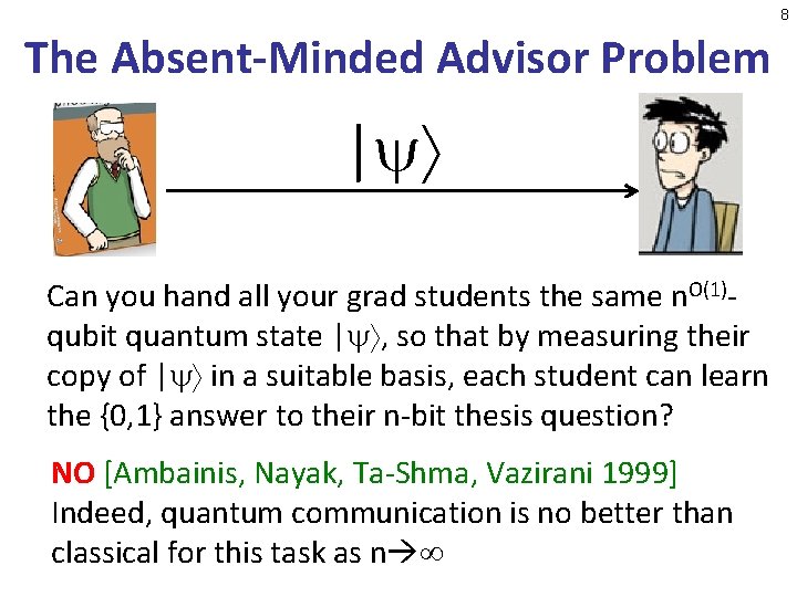
8 The Absent-Minded Advisor Problem | Can you hand all your grad students the same n. O(1)qubit quantum state | , so that by measuring their copy of | in a suitable basis, each student can learn the {0, 1} answer to their n-bit thesis question? NO [Ambainis, Nayak, Ta-Shma, Vazirani 1999] Indeed, quantum communication is no better than classical for this task as n

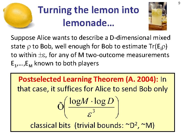
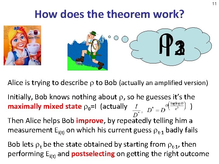
Turning the lemon into lemonade… Suppose Alice wants to describe a D-dimensional mixed state to Bob, well enough for Bob to estimate Tr(Ei ) to within , for any of M two-outcome measurements E 1, …, EM known to both players Postselected Learning Theorem (A. 2004): In that case, it suffices for Alice to send Bob only classical bits (trivial bounds: ~D 2, ~M) 9

| ALL YES/NO MEASUREMENTS PERFORMABLE USING ≤n 2 GATES 10

11 How does theorem work? I 321 Alice is trying to describe to Bob (actually an amplified version) Initially, Bob knows nothing about , so he guesses it’s the maximally mixed state 0=I (actually ) Then Alice helps Bob improve, by repeatedly telling him a measurement Ei(t) on which his current guess t-1 badly fails Bob lets t be the state obtained by starting from t-1, then performing Ei(t) and postselecting on getting the right outcome

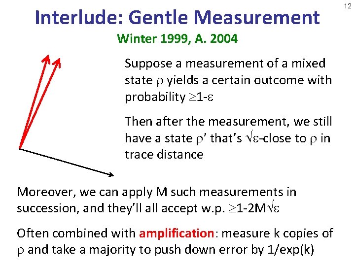
Interlude: Gentle Measurement Winter 1999, A. 2004 Suppose a measurement of a mixed state yields a certain outcome with probability 1 - Then after the measurement, we still have a state ’ that’s -close to in trace distance Moreover, we can apply M such measurements in succession, and they’ll accept w. p. 1 -2 M Often combined with amplification: measure k copies of and take a majority to push down error by 1/exp(k) 12

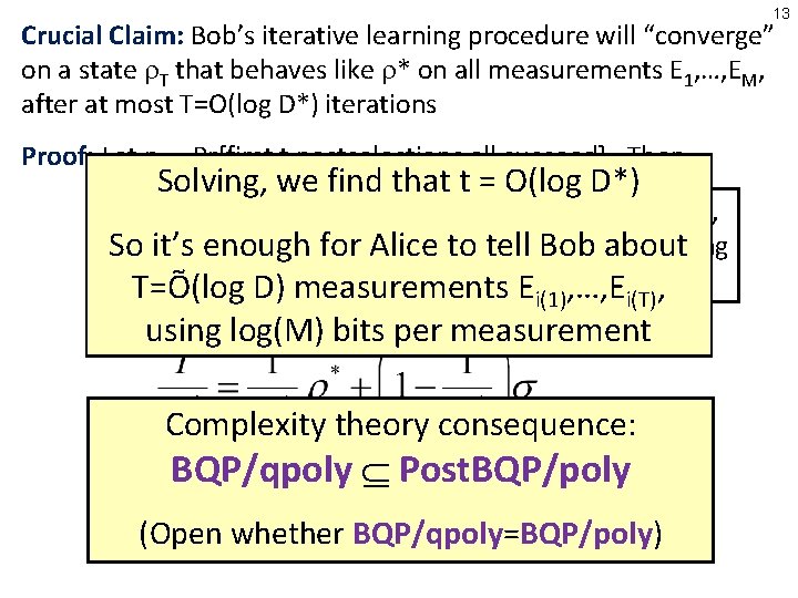
13 Crucial Claim: Bob’s iterative learning procedure will “converge” on a state T that behaves like * on all measurements E 1, …, EM, after at most T=O(log D*) iterations Proof: Let pt = Pr[first t postselections all succeed]. Then Solving, we find that t = O(log D*) If pt wasn’t less than, , learning So it’s enough for Alice tosay, tell(2/3)p Bob t-1 about would’ve ended!, T=Õ(log D) measurements E , …, E i(1) i(T) using log(M) bits per measurement Complexity theory consequence: BQP/qpoly Post. BQP/poly (Open whether BQP/qpoly=BQP/poly)

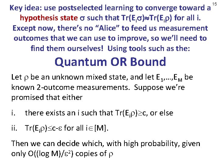
14 New Result [A. 2017]: “Shadow Tomography” Theorem: Let be an unknown D-dimensional state, and let E 1, …, EM be known 2 -outcome measurements. Suppose we want to know Tr(Ei ) to within additive error , for all i [M]. We can achieve this, with high probability, given only k copies of , where Open Problem: Dependence on D removable? Challenge: How to measure E 1, …, EM without destroying our few copies of in the process!

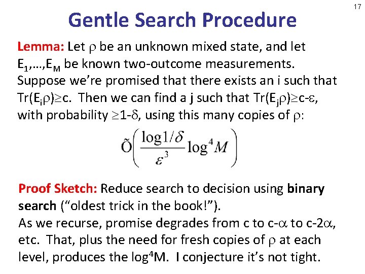
Key idea: use postselected learning to converge toward a hypothesis state such that Tr(Ei ) for all i. Except now, there’s no “Alice” to feed us measurement outcomes that we can use to improve, so we’ll need to find them ourselves! Using tools such as the: Quantum OR Bound Let be an unknown mixed state, and let E 1, …, EM be known 2 -outcome measurements. Suppose we’re promised that either i. there exists an i such that Tr(Ei ) c, or else ii. Tr(Ei ) c- for all i [M]. Then we can decide which, with high probability, given only O((log M)/ 2) copies of 15

16 [A. 2006] claimed a proof of the Quantum OR Bound, based on just applying amplified Ei’s in a random order [Harrow-Lin-Montanaro, SODA’ 2017] discovered an error in my proof—but also fixed it! They give two procedures, one of which is to prepare a control qubit in the state then repeatedly apply amplified Ei’s conditioned on the control qubit being |1 , while also periodically measuring the control qubit to see if it’s decohered (in which case we’re in case (ii)) Remains open whether my simpler procedure is also sound

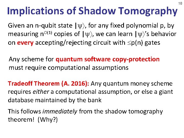
Gentle Search Procedure Lemma: Let be an unknown mixed state, and let E 1, …, EM be known two-outcome measurements. Suppose we’re promised that there exists an i such that Tr(Ei ) c. Then we can find a j such that Tr(Ej ) c- , with probability 1 - , using this many copies of : Proof Sketch: Reduce search to decision using binary search (“oldest trick in the book!”). As we recurse, promise degrades from c to c-2 , etc. That, plus the need for fresh copies of at each level, produces the log 4 M. I conjecture it’s not tight. 17

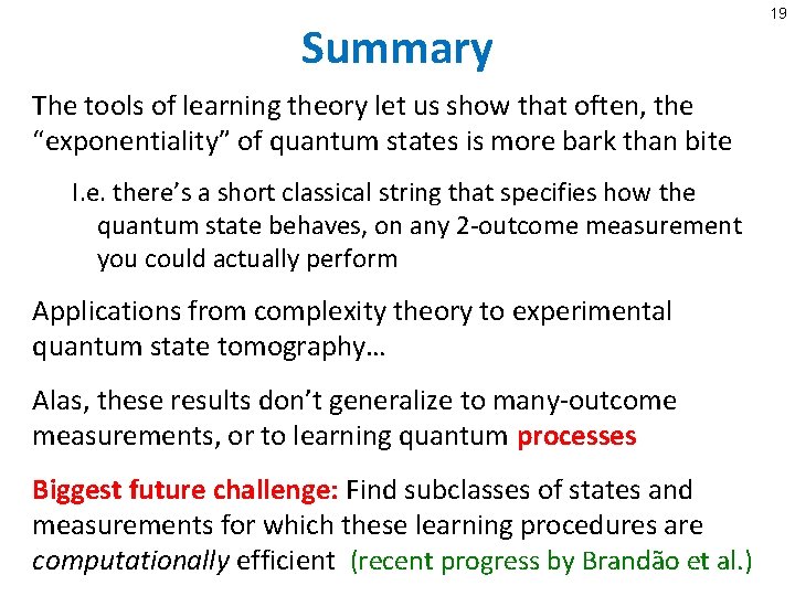
Implications of Shadow Tomography Given an n-qubit state | , for any fixed polynomial p, by measuring n. O(1) copies of | , we can learn | ’s behavior on every accepting/rejecting circuit with p(n) gates Any scheme for quantum software copy-protection must require computational assumptions Tradeoff Theorem (A. 2016): Any quantum money scheme requires either a computational assumption, or else a giant database maintained by the bank This follows immediately from the shadow tomography theorem! (Why? ) 18

Summary The tools of learning theory let us show that often, the “exponentiality” of quantum states is more bark than bite I. e. there’s a short classical string that specifies how the quantum state behaves, on any 2 -outcome measurement you could actually perform Applications from complexity theory to experimental quantum state tomography… Alas, these results don’t generalize to many-outcome measurements, or to learning quantum processes Biggest future challenge: Find subclasses of states and measurements for which these learning procedures are computationally efficient (recent progress by Brandão et al. ) 19

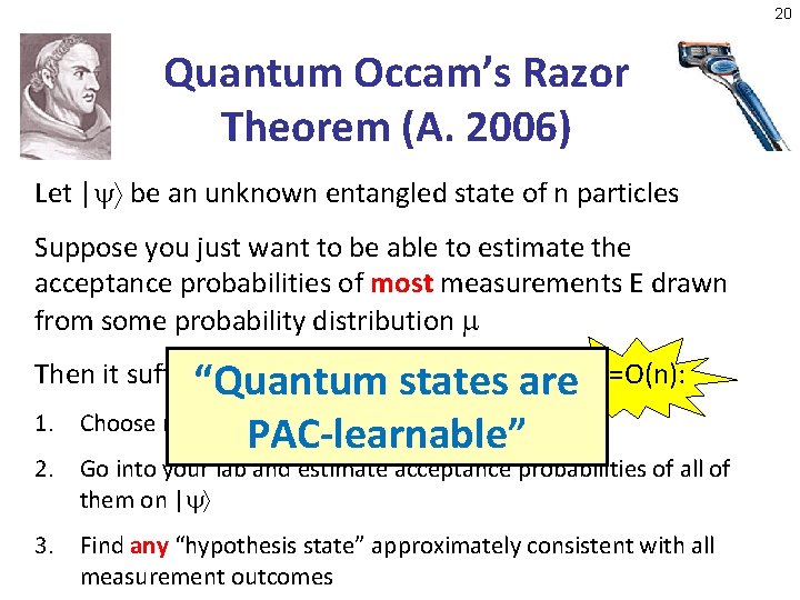
20 Quantum Occam’s Razor Theorem (A. 2006) Let | be an unknown entangled state of n particles Suppose you just want to be able to estimate the acceptance probabilities of most measurements E drawn from some probability distribution Then it suffices to do the following, for some “Quantum states are m=O(n): 1. Choose m measurements independently from PAC-learnable” 2. Go into your lab and estimate acceptance probabilities of all of them on | 3. Find any “hypothesis state” approximately consistent with all measurement outcomes

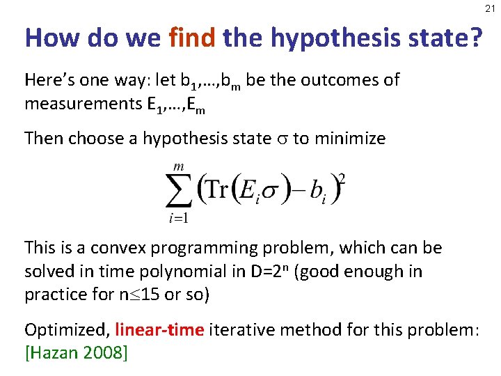
21 How do we find the hypothesis state? Here’s one way: let b 1, …, bm be the outcomes of measurements E 1, …, Em Then choose a hypothesis state to minimize This is a convex programming problem, which can be solved in time polynomial in D=2 n (good enough in practice for n 15 or so) Optimized, linear-time iterative method for this problem: [Hazan 2008]

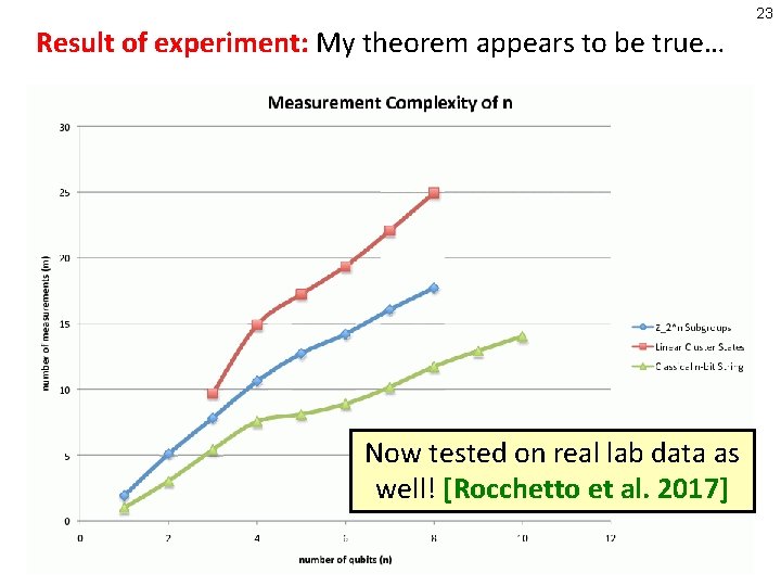
22 Numerical Simulation [A. -Dechter 2008] We implemented Hazan’s algorithm in MATLAB, and tested it on simulated quantum state data We studied how the number of sample measurements m needed for accurate predictions scales with the number of qubits n, for n≤ 10

23 Result of experiment: My theorem appears to be true… Now tested on real lab data as well! [Rocchetto et al. 2017]

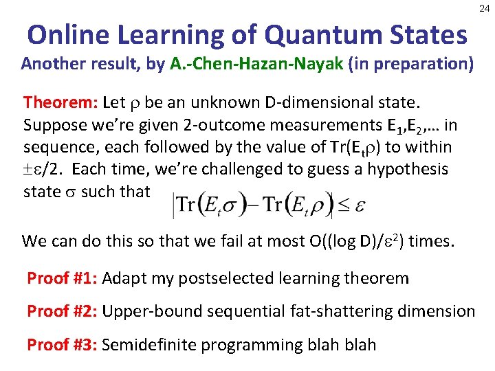
24 Online Learning of Quantum States Another result, by A. -Chen-Hazan-Nayak (in preparation) Theorem: Let be an unknown D-dimensional state. Suppose we’re given 2 -outcome measurements E 1, E 2, … in sequence, each followed by the value of Tr(Et ) to within /2. Each time, we’re challenged to guess a hypothesis state such that We can do this so that we fail at most O((log D)/ 2) times. Proof #1: Adapt my postselected learning theorem Proof #2: Upper-bound sequential fat-shattering dimension Proof #3: Semidefinite programming blah