Computation Quantum Theory and You Scott Aaronson UC

Computation, Quantum Theory, and You Scott Aaronson, UC Berkeley Qualifying Exam May 13, 2002

Talk Outline 1. 2. 3. 4. 5. Sermon Quantum Computing Overview Collision Lower Bound Dynamical Models Current and Future Work

1. Sermon

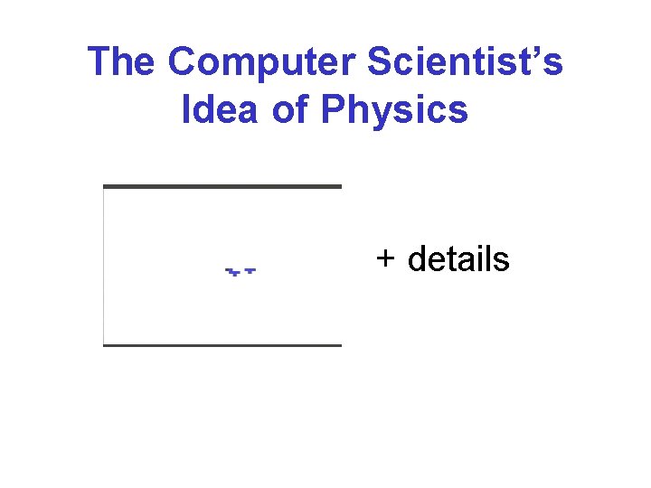
The Computer Scientist’s Idea of Physics + details

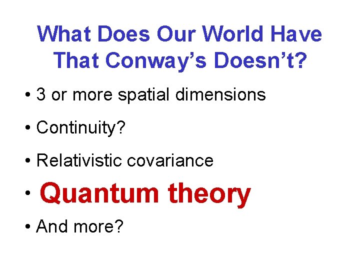
What Does Our World Have That Conway’s Doesn’t? • 3 or more spatial dimensions • Continuity? • Relativistic covariance • Quantum theory Quantum • And more?

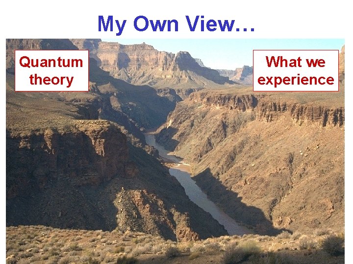
My Own View… Quantum theory What we experience

Research Goal Prove complexity results, focusing on quantum computing, that are motivated by this gap between physics and what we experience. (Disclaimer: I will not bridge the gap in my thesis. )

2. Quantum Computing

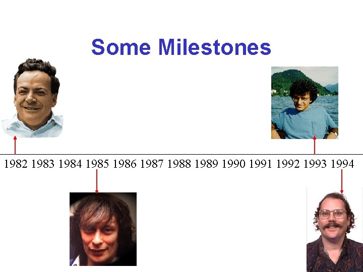
Some Milestones 1982 1983 1984 1985 1986 1987 1988 1989 1990 1991 1992 1993 1994

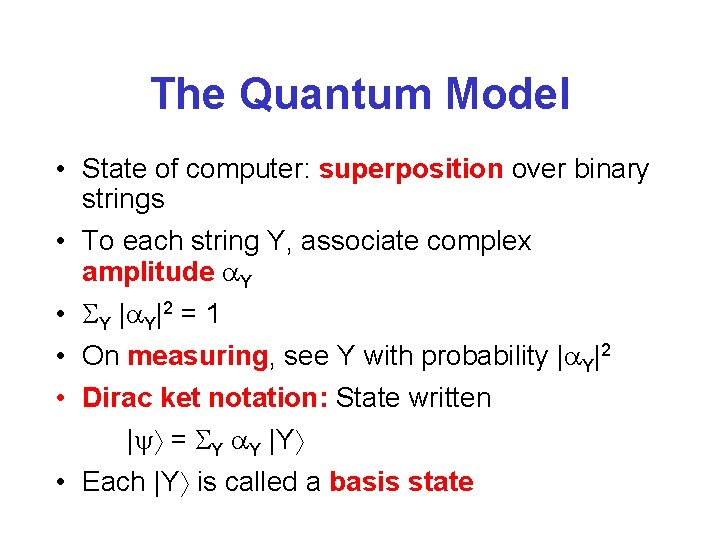
The Quantum Model • State of computer: superposition over binary strings • To each string Y, associate complex amplitude Y • Y | Y|2 = 1 • On measuring, see Y with probability | Y|2 • Dirac ket notation: State written | = Y Y |Y • Each |Y is called a basis state

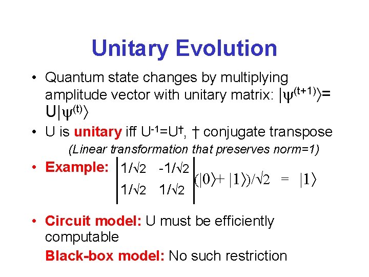
Unitary Evolution • Quantum state changes by multiplying amplitude vector with unitary matrix: | (t+1) = U| (t) • U is unitary iff U-1=U†, † conjugate transpose (Linear transformation that preserves norm=1) • Example: 1/ 2 -1/ 2 (|0 + |1 )/ 2 = |1 1/ 2 • Circuit model: U must be efficiently computable Black-box model: No such restriction

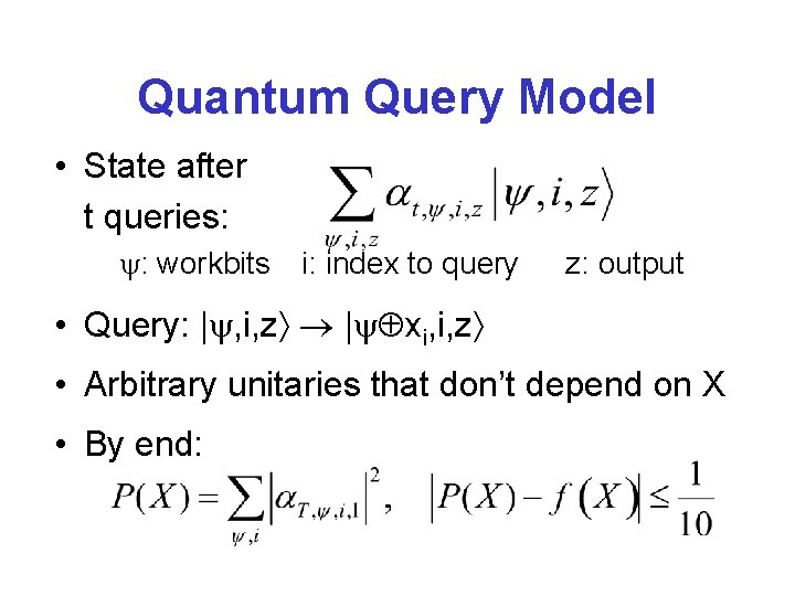
Quantum Query Model • State after t queries: : workbits i: index to query z: output • Query: | , i, z | xi, i, z • Arbitrary unitaries that don’t depend on X • By end:

3. Collision Lower Bound

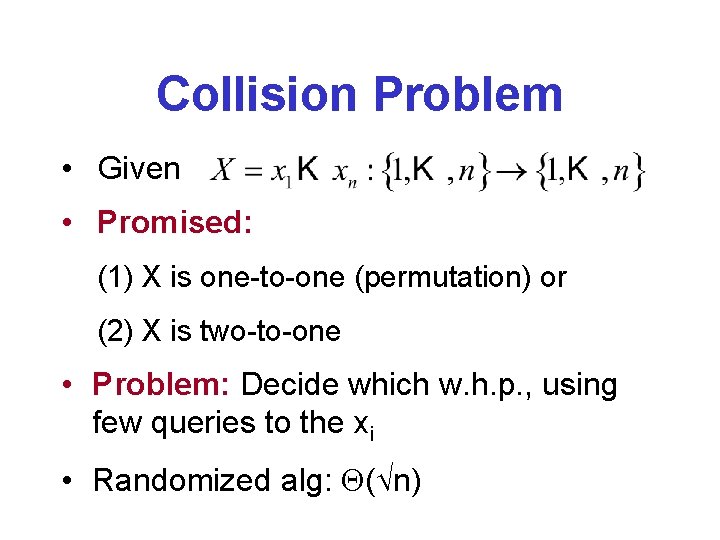
Collision Problem • Given • Promised: (1) X is one-to-one (permutation) or (2) X is two-to-one • Problem: Decide which w. h. p. , using few queries to the xi • Randomized alg: ( n)

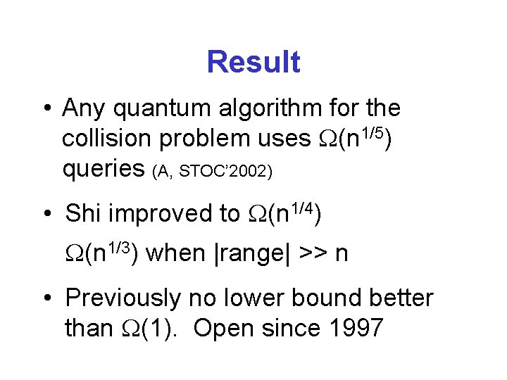
Result • Any quantum algorithm for the collision problem uses (n 1/5) queries (A, STOC’ 2002) • Shi improved to (n 1/4) (n 1/3) when |range| >> n • Previously no lower bound better than (1). Open since 1997

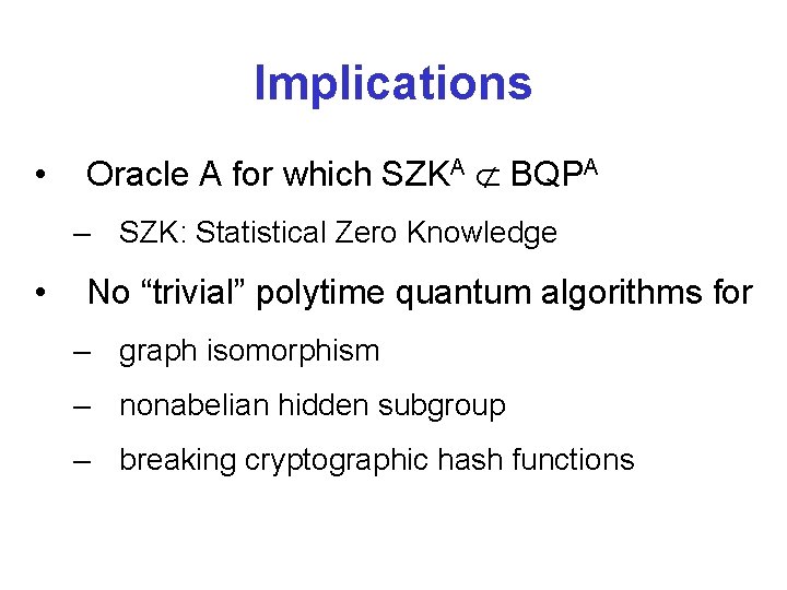
Implications • Oracle A for which SZKA BQPA – SZK: Statistical Zero Knowledge • No “trivial” polytime quantum algorithms for – graph isomorphism – nonabelian hidden subgroup – breaking cryptographic hash functions

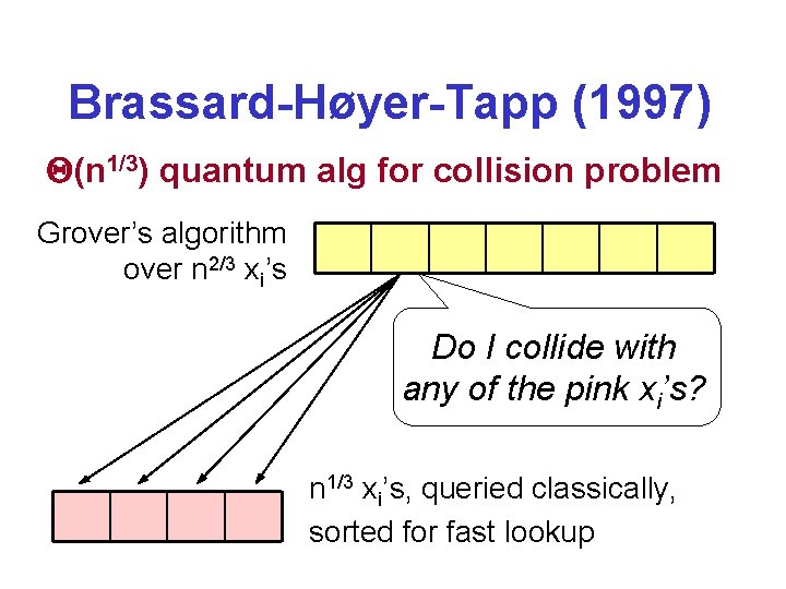
Brassard-Høyer-Tapp (1997) (n 1/3) quantum alg for collision problem Grover’s algorithm over n 2/3 xi’s Do I collide with any of the pink xi’s? n 1/3 xi’s, queried classically, sorted for fast lookup

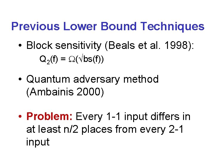
Previous Lower Bound Techniques • Block sensitivity (Beals et al. 1998): Q 2(f) = ( bs(f)) • Quantum adversary method (Ambainis 2000) • Problem: Every 1 -1 input differs in at least n/2 places from every 2 -1 input

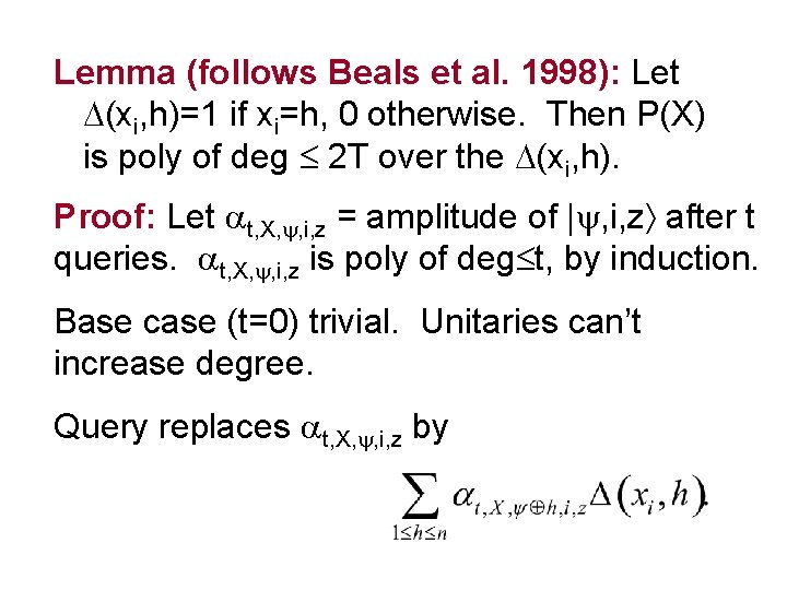
Lemma (follows Beals et al. 1998): Let (xi, h)=1 if xi=h, 0 otherwise. Then P(X) is poly of deg 2 T over the (xi, h). Proof: Let t, X, , i, z = amplitude of | , i, z after t queries. t, X, , i, z is poly of deg t, by induction. Base case (t=0) trivial. Unitaries can’t increase degree. Query replaces t, X, , i, z by

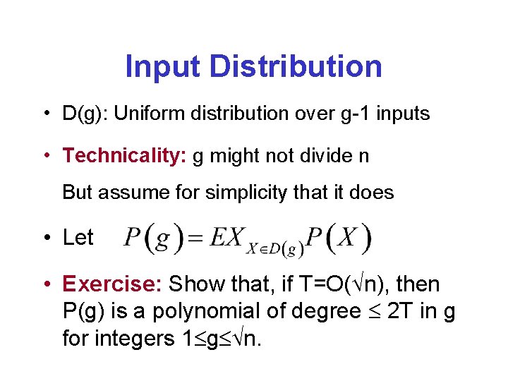
Input Distribution • D(g): Uniform distribution over g-1 inputs • Technicality: g might not divide n But assume for simplicity that it does • Let • Exercise: Show that, if T=O( n), then P(g) is a polynomial of degree 2 T in g for integers 1 g n.

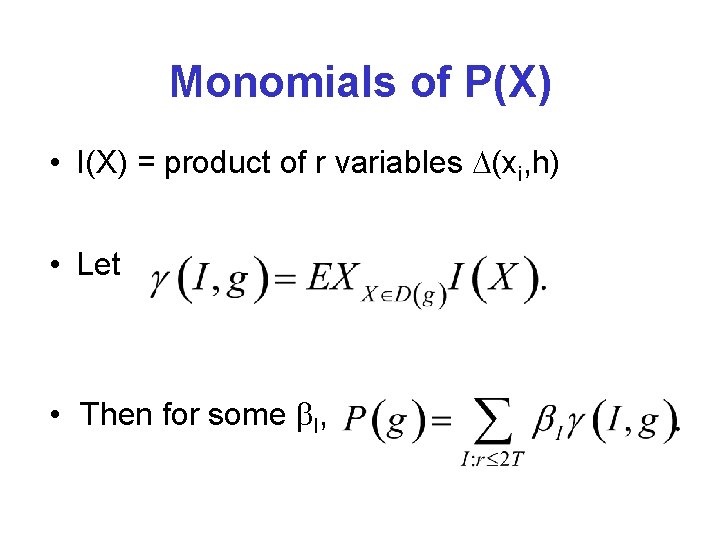
Monomials of P(X) • I(X) = product of r variables (xi, h) • Let • Then for some I,

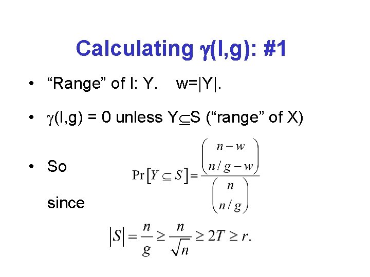
Calculating (I, g): #1 • “Range” of I: Y. w=|Y|. • (I, g) = 0 unless Y S (“range” of X) • So since

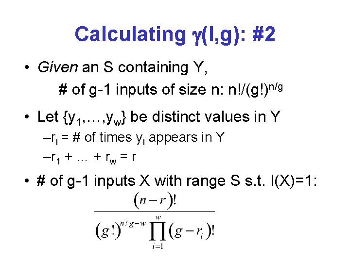
Calculating (I, g): #2 • Given an S containing Y, # of g-1 inputs of size n: n!/(g!)n/g • Let {y 1, …, yw} be distinct values in Y –ri = # of times yi appears in Y – r 1 + … + r w = r • # of g-1 inputs X with range S s. t. I(X)=1:

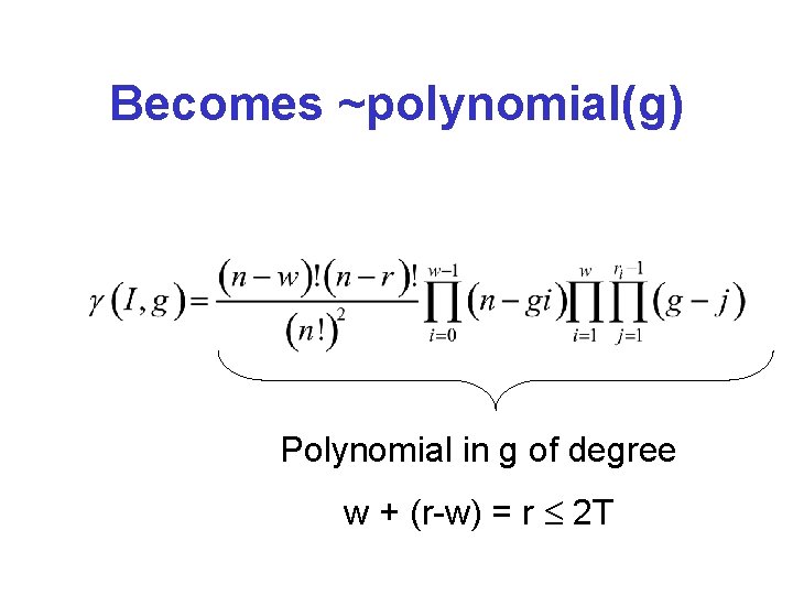
Becomes ~polynomial(g) Polynomial in g of degree w + (r-w) = r 2 T

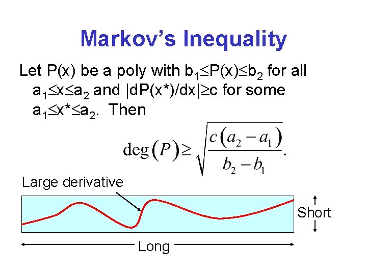
Markov’s Inequality Let P(x) be a poly with b 1 P(x) b 2 for all a 1 x a 2 and |d. P(x*)/dx| c for some a 1 x* a 2. Then Large derivative Short Long

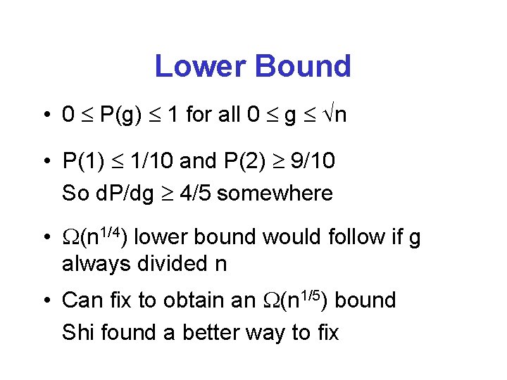
Lower Bound • 0 P(g) 1 for all 0 g n • P(1) 1/10 and P(2) 9/10 So d. P/dg 4/5 somewhere • (n 1/4) lower bound would follow if g always divided n • Can fix to obtain an (n 1/5) bound Shi found a better way to fix

4. Dynamical Models

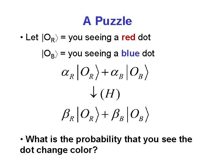
A Puzzle • Let |OR = you seeing a red dot |OB = you seeing a blue dot • What is the probability that you see the dot change color?

Why Is This An Issue? • Quantum theory says nothing about multiple-time or transition probabilities • Reply: “But we have no direct knowledge of the past anyway, just records” • But then what is a “prediction, ” or the “output of a computation, ” or the “utility of a decision”?

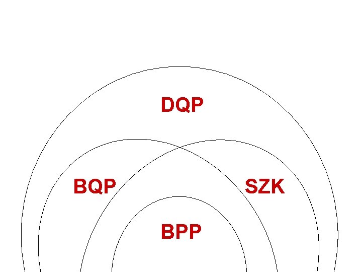
Results (submitted to PRL, quant-ph/0205059) • What if you could examine an observer’s entire history? Defined class DQP • Showed SZK DQP. Combined with collision bound, implies oracle A for which BQPA DQPA • Can search an N-element list in order N 1/3 steps, though not fewer

DQP BQP SZK BPP

5. Current and Future Work

BQP versus PH • Almost-complete (? !) joint work with Umesh • Conjecture: BQPA PHA for an oracle A (Best known: BQPA ( 2)A) • Use Recursive Fourier Sampling • Have reduced problem to generalizing the Razborov-Smolensky circuit lower bound • Need to show “replacer gates” don’t help us compute sum modulo 3

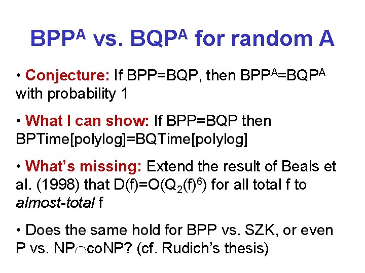
BPPA vs. BQPA for random A • Conjecture: If BPP=BQP, then BPPA=BQPA with probability 1 • What I can show: If BPP=BQP then BPTime[polylog]=BQTime[polylog] • What’s missing: Extend the result of Beals et al. (1998) that D(f)=O(Q 2(f)6) for all total f to almost-total f • Does the same hold for BPP vs. SZK, or even P vs. NP co. NP? (cf. Rudich’s thesis)

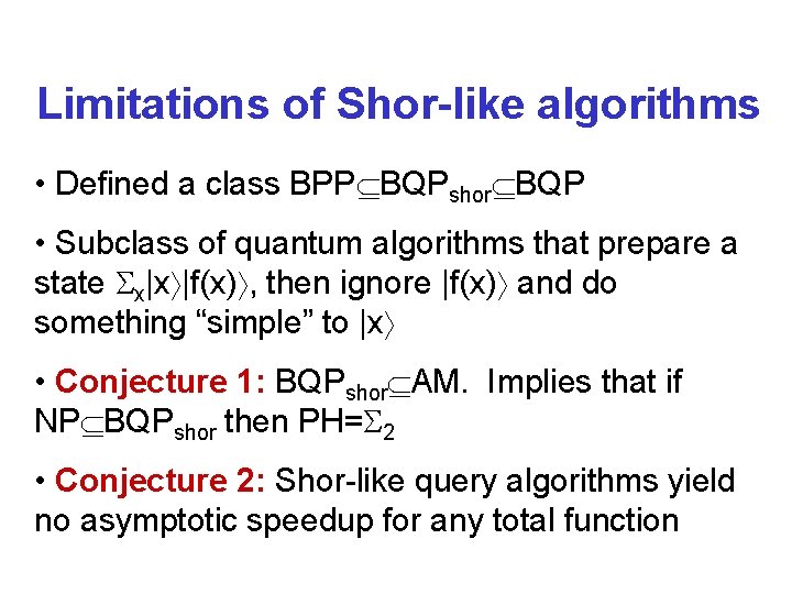
Limitations of Shor-like algorithms • Defined a class BPP BQPshor BQP • Subclass of quantum algorithms that prepare a state x|x |f(x) , then ignore |f(x) and do something “simple” to |x • Conjecture 1: BQPshor AM. Implies that if NP BQPshor then PH= 2 • Conjecture 2: Shor-like query algorithms yield no asymptotic speedup for any total function

Physics Modulo Complexity Assumptions • Can some version of M-theory decide SAT? (cf. Preskill’s talk) If so, move on to the next version! • “Anthropic computer” for solving NP-complete problems efficiently • Stupid question: Why can’t I just “will” myself to solve NP-complete problems? (Or generate truly random sequences? )

Postulate: No matter who you are, someone can give you a 3 SAT instance that you can’t decide with probability ½+. What constraints does that impose?