Math Tutorial for computer vision Draft KH Wong

Math Tutorial for computer vision (Draft) KH Wong Face recognition & detection using PCA v. 0. a 1

Overview • Basic geometry – 2 D – 3 D • Linear Algebra – Eigen values and vectors – Ax=b and SVD • Non-linear optimization – Jacobian – Probability vs. Face likelihood (maximum likelihood) recognition & detection using PCA v. 0. a 2

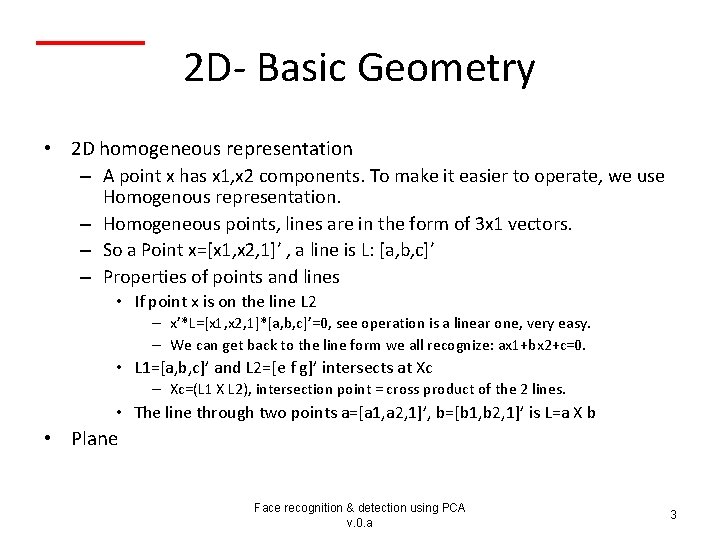
2 D- Basic Geometry • 2 D homogeneous representation – A point x has x 1, x 2 components. To make it easier to operate, we use Homogenous representation. – Homogeneous points, lines are in the form of 3 x 1 vectors. – So a Point x=[x 1, x 2, 1]’ , a line is L: [a, b, c]’ – Properties of points and lines • If point x is on the line L 2 – x’*L=[x 1, x 2, 1]*[a, b, c]’=0, see operation is a linear one, very easy. – We can get back to the line form we all recognize: ax 1+bx 2+c=0. • L 1=[a, b, c]’ and L 2=[e f g]’ intersects at Xc – Xc=(L 1 X L 2), intersection point = cross product of the 2 lines. • The line through two points a=[a 1, a 2, 1]’, b=[b 1, b 2, 1]’ is L=a X b • Plane Face recognition & detection using PCA v. 0. a 3

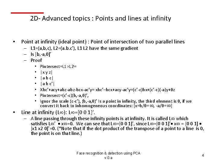
2 D- Advanced topics : Points and lines at infinity • Point at infinity (ideal point) : Point of intersection of two parallel lines – L 1=(a, b, c), L 2=(a. b. c’), L 1 L 2 have the same gradient – Is [b, -a, 0]’ – Proof • • Pintersect=L 1 L 2= |x y z| |a b c’| Xbc’+acy+abz-bcx-ac’y= xbc’–bcx+acy-ac’y=(c’-c)bx+(c’-c)(-a)y+0 z Pintersect=(c’-c)(b, -a, 0)’, Ignor the scale (c-c’), (b, -a, 0)’ Is a point in infinity, the third element is 0, if we convert it back to inhomogeneous coordinates: [x=b/0= , -a/0= ] Line at infinity (L ): L =[0 0 1]’. – A line passing through these infinity points is at infinity. It is called L which satisfies L ’ x =0. We can see that L =[0 0 1]’, since L =[0 0 1]’ x = [0 0 1] [x 1 x 2 0]’=0. (*Note that if the dot product of the transpose of a point to a line is 0, the point is on that line. ) Face recognition & detection using PCA v. 0. a 4

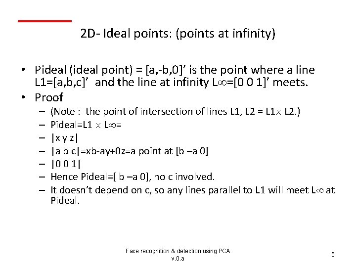
2 D- Ideal points: (points at infinity) • Pideal (ideal point) = [a, -b, 0]’ is the point where a line L 1=[a, b, c]’ and the line at infinity L =[0 0 1]’ meets. • Proof – – – – (Note : the point of intersection of lines L 1, L 2 = L 1 L 2. ) Pideal=L 1 L = |x y z| |a b c|=xb-ay+0 z=a point at [b –a 0] |0 0 1| Hence Pideal=[ b –a 0], no c involved. It doesn’t depend on c, so any lines parallel to L 1 will meet L at Pideal. Face recognition & detection using PCA v. 0. a 5

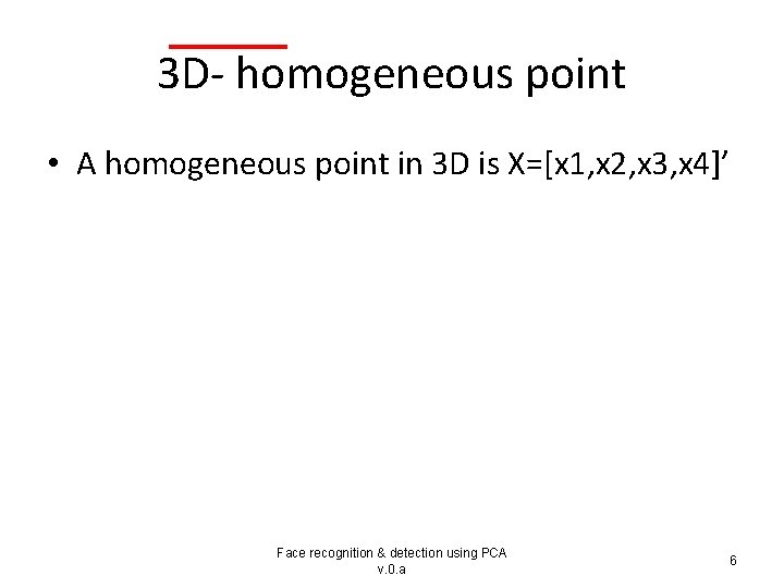
3 D- homogeneous point • A homogeneous point in 3 D is X=[x 1, x 2, x 3, x 4]’ Face recognition & detection using PCA v. 0. a 6

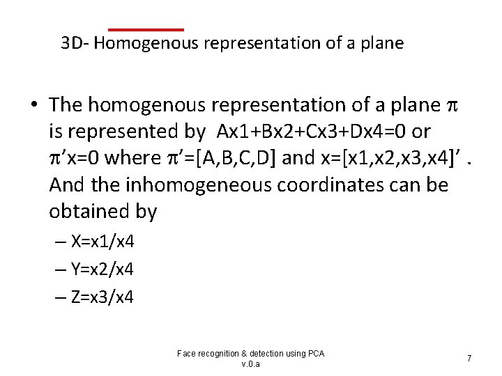
3 D- Homogenous representation of a plane • The homogenous representation of a plane is represented by Ax 1+Bx 2+Cx 3+Dx 4=0 or ’x=0 where ’=[A, B, C, D] and x=[x 1, x 2, x 3, x 4]’. And the inhomogeneous coordinates can be obtained by – X=x 1/x 4 – Y=x 2/x 4 – Z=x 3/x 4 Face recognition & detection using PCA v. 0. a 7

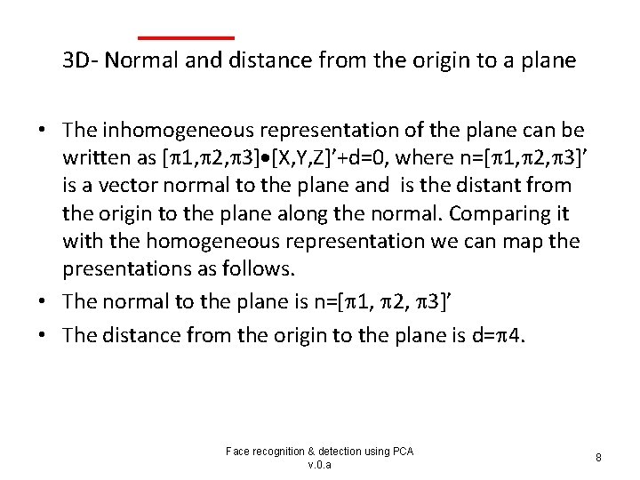
3 D- Normal and distance from the origin to a plane • The inhomogeneous representation of the plane can be written as [ 1, 2, 3] [X, Y, Z]’+d=0, where n=[ 1, 2, 3]’ is a vector normal to the plane and is the distant from the origin to the plane along the normal. Comparing it with the homogeneous representation we can map the presentations as follows. • The normal to the plane is n=[ 1, 2, 3]’ • The distance from the origin to the plane is d= 4. Face recognition & detection using PCA v. 0. a 8

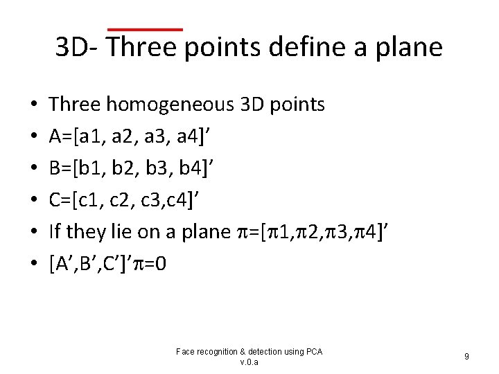
3 D- Three points define a plane • • • Three homogeneous 3 D points A=[a 1, a 2, a 3, a 4]’ B=[b 1, b 2, b 3, b 4]’ C=[c 1, c 2, c 3, c 4]’ If they lie on a plane =[ 1, 2, 3, 4]’ [A’, B’, C’]’ =0 Face recognition & detection using PCA v. 0. a 9

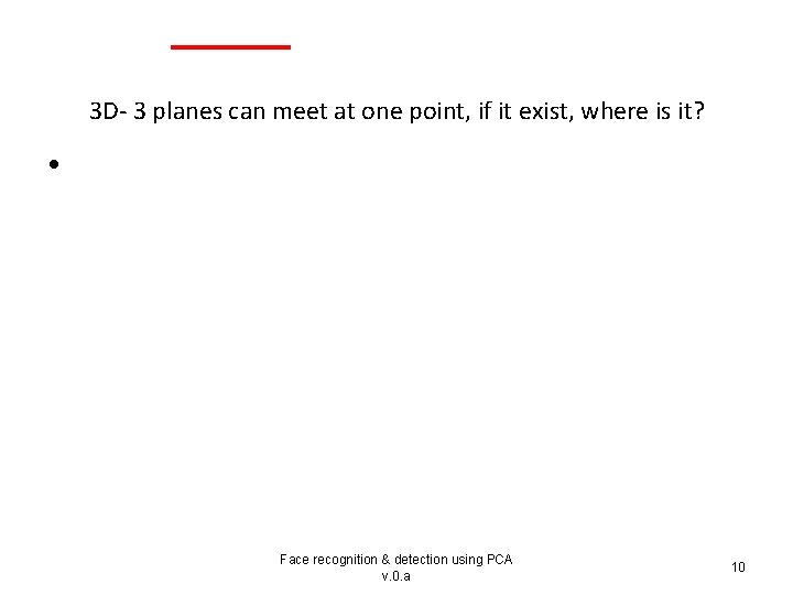
3 D- 3 planes can meet at one point, if it exist, where is it? • Face recognition & detection using PCA v. 0. a 10

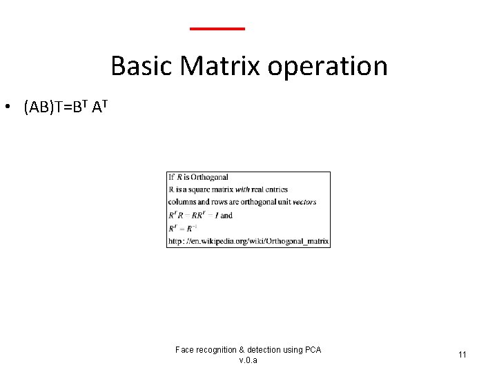
Basic Matrix operation • (AB)T=BT AT Face recognition & detection using PCA v. 0. a 11

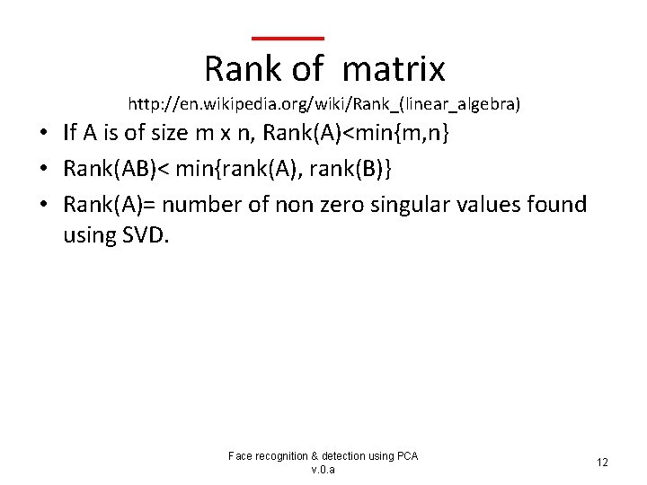
Rank of matrix http: //en. wikipedia. org/wiki/Rank_(linear_algebra) • If A is of size m x n, Rank(A)<min{m, n} • Rank(AB)< min{rank(A), rank(B)} • Rank(A)= number of non zero singular values found using SVD. Face recognition & detection using PCA v. 0. a 12

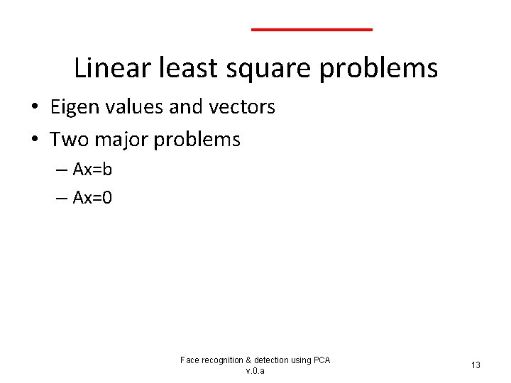
Linear least square problems • Eigen values and vectors • Two major problems – Ax=b – Ax=0 Face recognition & detection using PCA v. 0. a 13

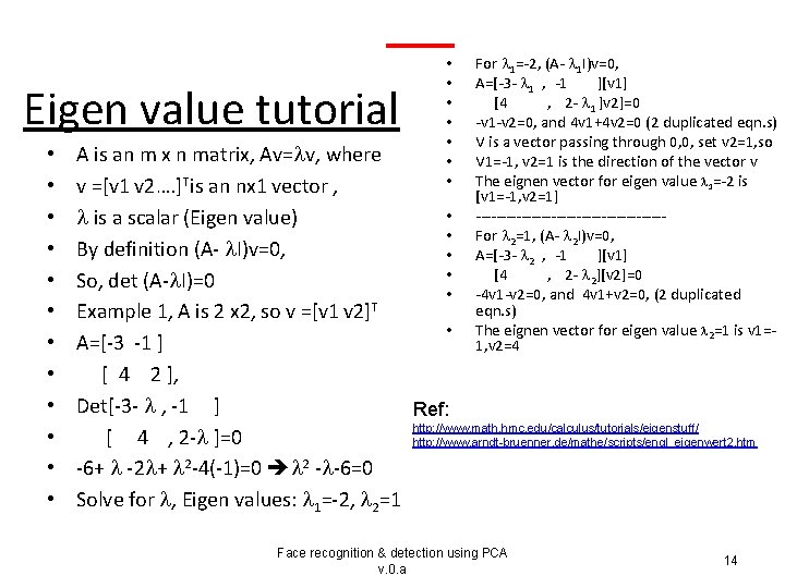
Eigen value tutorial • • • • • For 1=-2, (A- 1 I)v=0, A=[-3 - 1 , -1 ][v 1] [4 , 2 - 1 ]v 2]=0 -v 1 -v 2=0, and 4 v 1+4 v 2=0 (2 duplicated eqn. s) V is a vector passing through 0, 0, set v 2=1, so V 1=-1, v 2=1 is the direction of the vector v The eignen vector for eigen value 1=-2 is [v 1=-1, v 2=1] -------------------For 2=1, (A- 2 I)v=0, A=[-3 - 2 , -1 ][v 1] [4 , 2 - 2][v 2]=0 -4 v 1 -v 2=0, and 4 v 1+v 2=0, (2 duplicated eqn. s) The eignen vector for eigen value 2=1 is v 1=1, v 2=4 A is an m x n matrix, Av= v, where v =[v 1 v 2…. ]Tis an nx 1 vector , • is a scalar (Eigen value) • By definition (A- I)v=0, • • So, det (A- I)=0 • T Example 1, A is 2 x 2, so v =[v 1 v 2] • A=[-3 -1 ] [ 4 2 ], Det[-3 - , -1 ] Ref: http: //www. math. hmc. edu/calculus/tutorials/eigenstuff/ [ 4 , 2 - ]=0 http: //www. arndt-bruenner. de/mathe/scripts/engl_eigenwert 2. htm -6+ -2 + 2 -4(-1)=0 2 - -6=0 Solve for , Eigen values: 1=-2, 2=1 Face recognition & detection using PCA v. 0. a 14

Eigen value tutorial • • Example 2, m=2, n=2 A=[1 13 13 1], Det[1 - , 13 13 , 1 - ]=0 (1 - )2 -2(1 - )+132=0 Solve for , solutions: 1=-12, 2=14 • • for Eigenvalue -12: Eigenvector: [ -1 ; 1 ] • • for Eigenvalue 14: Eigenvector: [ 1 ; 1 ] Ref: Check the answer using http: //www. arndt-bruenner. de/mathe/scripts/engl_eigenwert 2. htm Face recognition & detection using PCA v. 0. a 15

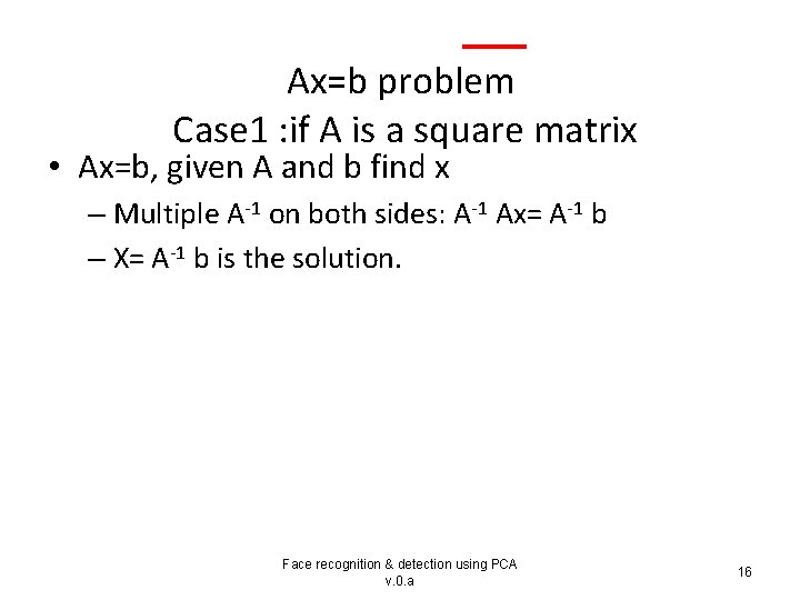
Ax=b problem Case 1 : if A is a square matrix • Ax=b, given A and b find x – Multiple A-1 on both sides: A-1 Ax= A-1 b – X= A-1 b is the solution. Face recognition & detection using PCA v. 0. a 16

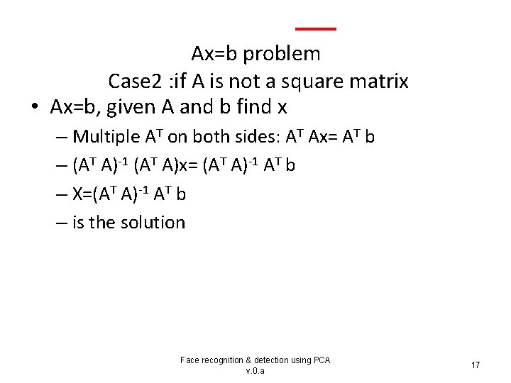
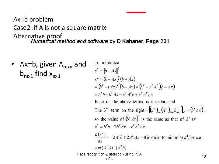
Ax=b problem Case 2 : if A is not a square matrix • Ax=b, given A and b find x – Multiple AT on both sides: AT Ax= AT b – (AT A)-1 (AT A)x= (AT A)-1 AT b – X=(AT A)-1 AT b – is the solution Face recognition & detection using PCA v. 0. a 17

Ax=b problem Case 2 : if A is not a square matrix Alternative proof Numerical method and software by D Kahaner, Page 201 • Ax=b, given Amxn and bmx 1 find xnx 1 Face recognition & detection using PCA v. 0. a 18

Solve Ax=0 • To solve Ax=0, Homogeneous systems – One solution is x=0, but it is trivial and no use. – We need another method, SVD (Singular value decomposition) Face recognition & detection using PCA v. 0. a 19

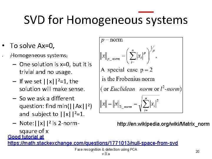
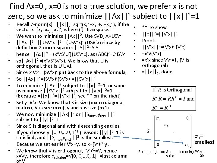
SVD for Homogeneous systems • To solve Ax=0, • Homogeneous systems) ( – One solution is x=0, but it is trivial and no usage. – If we set ||x||2=1, the solution will make sense. – So we ask a different question: find min(||Ax||2) and subject to ||x||2=1. – Note: ||x||2 is 2 -normsqaure of x http: //en. wikipedia. org/wiki/Matrix_norm Good tutorial at https: //math. stackexchange. com/questions/1771013/null-space-from-svd Face recognition & detection using PCA v. 0. a 20

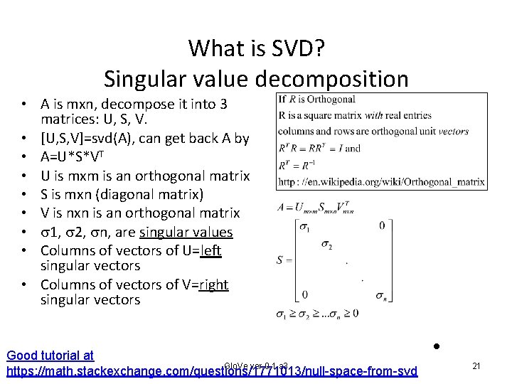
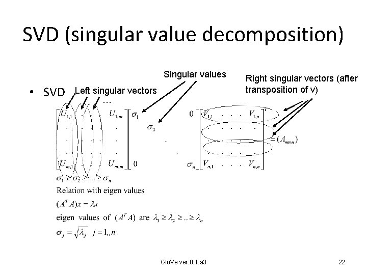
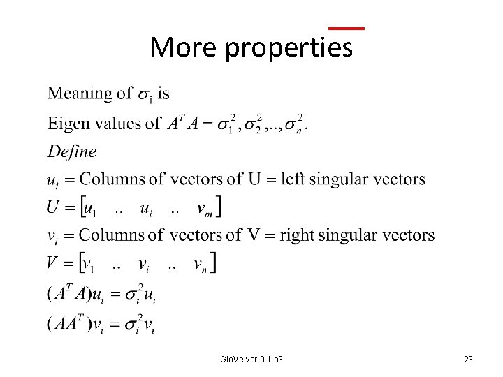
What is SVD? Singular value decomposition • A is mxn, decompose it into 3 matrices: U, S, V. • [U, S, V]=svd(A), can get back A by • A=U*S*VT • U is mxm is an orthogonal matrix • S is mxn (diagonal matrix) • V is nxn is an orthogonal matrix • 1, 2, n, are singular values • Columns of vectors of U=left singular vectors • Columns of vectors of V=right singular vectors Good tutorial at Glo. Ve ver. 0. 1. a 3 https: //math. stackexchange. com/questions/1771013/null-space-from-svd • 21

SVD (singular value decomposition) Singular values • SVD Left singular vectors … Glo. Ve ver. 0. 1. a 3 Right singular vectors (after transposition of v) 22

More properties Glo. Ve ver. 0. 1. a 3 23

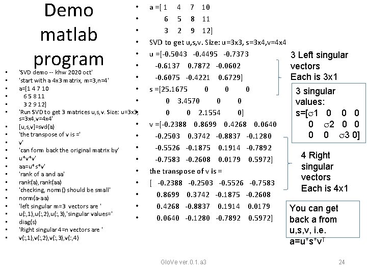
• • • • • • Demo matlab program • • • 'SVD demo -- khw 2020 oct' • 'start with a 4 x 3 matrix, m=3, n=4' a=[1 4 7 10 • 6 5 8 11 • 3 2 9 12] 'Run SVD to get 3 matrices u, s, v. Size: u=3 x 3, • s=3 x 4, v=4 x 4' • [u, s, v]=svd(a) 'the transpose of v is =' • v' • 'can form back the original matrix by’ u*v*v' • aa=u*s*v' • 'rank of a and aa' rank(a), rank(aa) • 'checking, norm() should be small' • norm(a-aa) 'left singular m=3 vectors are ' • u(: , 1), u(: , 2), u(: , 3), 'singular values=' • diag(s) a =[ 1 4 7 10 6 5 8 11 3 2 9 12] SVD to get u, s, v. Size: u=3 x 3, s=3 x 4, v=4 x 4 u =[-0. 5043 -0. 4495 -0. 7373 -0. 6137 0. 7872 -0. 0602 -0. 6075 -0. 4221 0. 6729] s =[25. 1675 0 0 3. 4570 0 0 2. 1554 0] v =[-0. 2388 0. 8699 0. 4268 0. 0640 -0. 2503 0. 3742 -0. 8837 -0. 1280 -0. 5526 -0. 1875 0. 1914 -0. 7892 -0. 7583 -0. 2608 0. 0179 0. 5972] the transpose of v is = [ -0. 2388 -0. 2503 -0. 5526 -0. 7583 0. 8699 0. 3742 -0. 1875 -0. 2608 0. 4268 -0. 8837 0. 1914 0. 0179 0. 0640 -0. 1280 -0. 7892 0. 5972] 'Right singular 4=n vectors are ' v(: , 1), v(: , 2), v(: , 3), v(: , 4) Glo. Ve ver. 0. 1. a 3 3 Left singular vectors Each is 3 x 1 3 singular values: s=[ 1 0 0 2 0 0 3 0] 4 Right singular vectors Each is 4 x 1 You can get back a from u, s, v, i. e. a=u*s*v. T 24

Find Ax=0 , x=0 is not a true solution, we prefer x is not zero, so we ask to minimize ||Ax||2 subject to ||x||2=1 • • • • Recall 2 -norm(x)= ||x||2=sqrt(x 12+. . +xn 2 ), if the vector x=[x 1, x 2, . . , xn]’, where (’)=transpose. We want to minimize ||Ax||2. Use SVD, A=USV’ ||Ax||2 =||USV’x||2 = (USV’x)’ (USV’x) since by definition 2 -norm-sqaure: ||Y||2=Y’Y hence ||Ax||2 = (x’VS’U’)(USV’x), as (ABC)’=C’B’A’ so||Ax||2 =(x’VS’SV’x). We know that U is orthogonal, that is U’U=1 Since x’VS’= (SV’x)’ put back to the above formula, So ||Ax||2 =(SV’x)’(SV’x) =||SV’x||2 To minimize ||Ax||2 subject to ||x||2=1, or same as minimize ||SV’x||2 subject to ||V’x||2=1 (because =||x||2=||V’x||2, see ** on the right) Set y=V’x. We know that S is size (mxn) (diagonal matrix), V is size (nxn), y and x is size (nx 1). We now minimize ||Ax||2 or ||S(mxn)y(nx 1)||2 subject to ||y||2=1 Since S is diagonal and with descending entries If you choose y=[0, 0, . . , 0, 1]T (reason: ||y||2=1 is satisfied, and ||S(mxn)y(nx 1)||2 is the smallest. Because we set earlier V’x=y, so x=(V’)-1 y. We know that V is orthogonal, (V’)-1=V, hence x=Vy, therefore xsolution=V[0, 0, . . , 0, 1]T =last column of V • • ** To show ||x||2=||V’x||2 Proof: ||V’x||2=(V’x)’ (V’x) =x’V(V’x) =x’x since VV’=I , (V is orthogonal) =||x||2, done n = smallest Face recognition & detection using PCA 25 v. 0. a

• Nonlinear leave square Jacobian Face recognition & detection using PCA v. 0. a 26

Non-linear optimization • To be added Face recognition & detection using PCA v. 0. a 27

Some math background on statistics 1. Mean, Variance/ standard deviation 2. Covariance and Covariance matrix 3. Eigen value and Eigen vector Face recognition & detection using PCA v. 0. a 28

Mathematical methods in Statistics 1. Mean, variance (var) and standard_deviation (std), Face recognition & detection using PCA v. 0. a 29

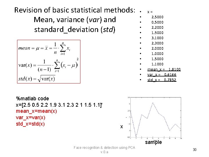
Revision of basic statistical methods: Mean, variance (var) and standard_deviation (std) %matlab code x=[2. 5 0. 5 2. 2 1. 9 3. 1 2. 3 2 1 1. 5 1. 1]' mean_x=mean(x) var_x=var(x) std_x=std(x) • • • • x= 2. 5000 0. 5000 2. 2000 1. 9000 3. 1000 2. 3000 2. 0000 1. 5000 1. 1000 mean_x = 1. 8100 var_x = 0. 6166 std_x = 0. 7852 x sample Face recognition & detection using PCA v. 0. a 30

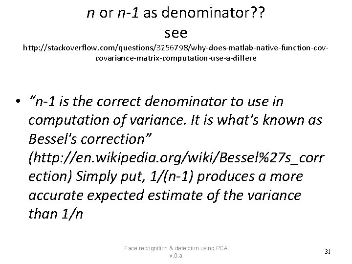
n or n-1 as denominator? ? see http: //stackoverflow. com/questions/3256798/why-does-matlab-native-function-covcovariance-matrix-computation-use-a-differe • “n-1 is the correct denominator to use in computation of variance. It is what's known as Bessel's correction” (http: //en. wikipedia. org/wiki/Bessel%27 s_corr ection) Simply put, 1/(n-1) produces a more accurate expected estimate of the variance than 1/n Face recognition & detection using PCA v. 0. a 31

Class exercise 1 By computer (Matlab) • • x=[1 3 5 10 12]' mean(x) var(x) std(x) Mean(x) = 6. 2000 Variance(x)= 21. 7000 Stand deviation = 4. 6583 By and • • x=[1 3 5 10 12]' mean= Variance= Standard deviation= %class exercise 1 x=[1 3 5 10 12]' mean(x) var(x) std(x) 32 Face recognition & detection using PCA v. 0. a

Answer 1: By computer (Matlab) • • x=[1 3 5 10 12]' mean(x) var(x) std(x) Mean(x) = 6. 2000 Variance(x)= 21. 7000 Stand deviation = 4. 6583 By and x=[1 3 5 10 12]' mean=(1+3+5+10+12)/5 =6. 2 Variance=((1 -6. 2)^2+(36. 2)^2+(5 -6. 2)^2+(106. 2)^2+(12 -6. 2)^2)/(51)=21. 7 • Standard deviation= sqrt(21. 7)= 4. 6583 • • Face recognition & detection using PCA v. 0. a 33

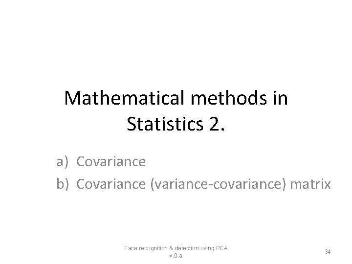
Mathematical methods in Statistics 2. a) Covariance b) Covariance (variance-covariance) matrix Face recognition & detection using PCA v. 0. a 34

Part 2 a: Covariance [see wolfram mathworld] http: //mathworld. wolfram. com/ • “Covariance is a measure of the extent to which corresponding elements from two sets of ordered data move in the same direction. ” • http: //stattrek. com/matrix-algebra/variance. aspx Face recognition & detection using PCA v. 0. a 35

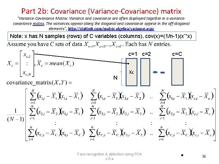
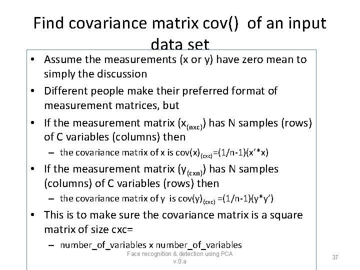
Part 2 b: Covariance (Variance-Covariance) matrix ”Variance-Covariance Matrix: Variance and covariance are often displayed together in a variancecovariance matrix. The variances appear along the diagonal and covariance appear in the off-diagonal elements”, http: //stattrek. com/matrix-algebra/variance. aspx Note: x has N samples (rows) of C variables (columns), cov(x)=(1/n-1)(x’*x) c=1 c=2 N c=C Xc Face recognition & detection using PCA v. 0. a • 36

Find covariance matrix cov() of an input data set • Assume the measurements (x or y) have zero mean to simply the discussion • Different people make their preferred format of measurement matrices, but • If the measurement matrix (x(nxc)) has N samples (rows) of C variables (columns) then – the covariance matrix of x is cov(x)(cxc)=(1/n-1)(x’*x) • If the measurement matrix (y(cxn)) has N samples (columns) of C variables (rows) then – the covariance matrix of y is cov(y)(cxc) =(1/n-1)(y*y’) • This is to make sure the covariance matrix is a square matrix of size cxc= – number_of_variables x number_of_variables Face recognition & detection using PCA v. 0. a 37

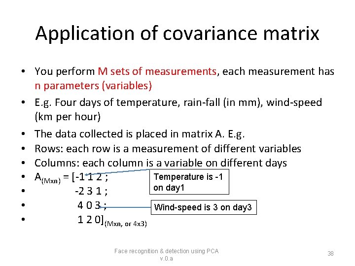
Application of covariance matrix • You perform M sets of measurements, each measurement has n parameters (variables) • E. g. Four days of temperature, rain-fall (in mm), wind-speed (km per hour) • The data collected is placed in matrix A. E. g. • Rows: each row is a measurement of different variables • Columns: each column is a variable on different days Temperature is -1 • A(Mxn) = [-1 1 2 ; on day 1 • -2 3 1 ; • 403; Wind-speed is 3 on day 3 • 1 2 0](Mxn, or 4 x 3) Face recognition & detection using PCA v. 0. a 38

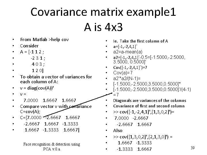
Covariance matrix example 1 A is 4 x 3 • • • • From Matlab >help cov Consider A = [-1 1 2 ; -2 3 1 ; 403; 1 2 0] To obtain a vector of variances for each column of A: v = diag(cov(A))' v= 7. 0000 1. 6667 Compare vector v with covariance C=cov(A); C=[7. 0000 -2. 6667 1. 6667 -1. 3333 1. 6667] Face recognition & detection using PCA v. 0. a • • • • • Ie. Take the first column of A a=[-1, -2, 4, 1]’ a 2=a-mean(a) a 2=[-1, -2, 4, 1]’-0. 5=[-1. 5000, -2. 5000, 3. 5000, 0. 5000]’ Cov([-1, -2, 4, 1]’)=7 Cov(a)=7 a 2’*a 2/(N-1)= [-1. 5000, -2. 5000, 3. 5000, 0. 5000]* [-1. 5000, -2. 5000, 3. 5000, 0. 5000]’/(4 -1) =7 Diagonals are variances of the columns Covariance of first and second column >> cov([-1, -2, 4, 1]', [1, 3, 0, 2]')= 7. 0000 -2. 6667 1. 6667 Also >> cov([1, 3, 0, 2]', [2, 1, 3, 0]') = 1. 6667 -1. 3333 1. 6667 39

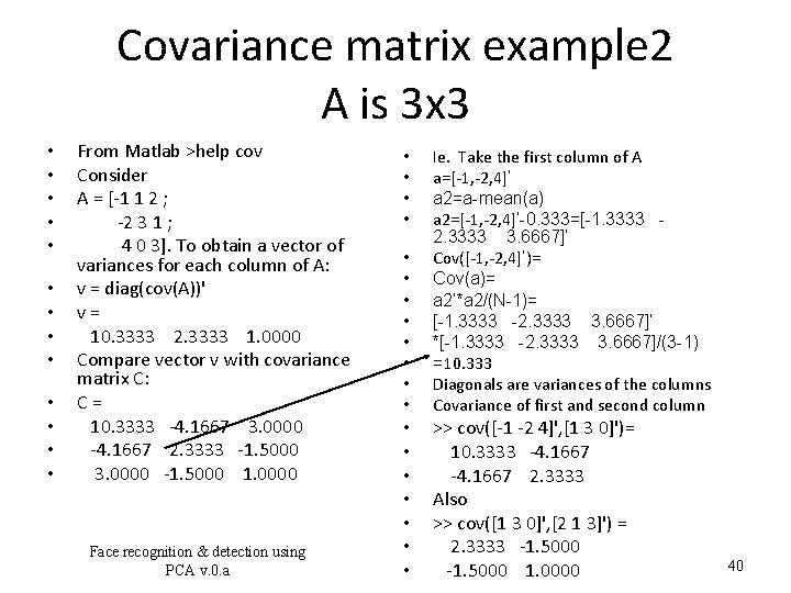
Covariance matrix example 2 A is 3 x 3 • • • • From Matlab >help cov Consider A = [-1 1 2 ; -2 3 1 ; 4 0 3]. To obtain a vector of variances for each column of A: v = diag(cov(A))' v= 10. 3333 2. 3333 1. 0000 Compare vector v with covariance matrix C: C= 10. 3333 -4. 1667 3. 0000 -4. 1667 2. 3333 -1. 5000 3. 0000 -1. 5000 1. 0000 Face recognition & detection using PCA v. 0. a • • • • • Ie. Take the first column of A a=[-1, -2, 4]’ a 2=a-mean(a) a 2=[-1, -2, 4]’-0. 333=[-1. 3333 2. 3333 3. 6667]’ Cov([-1, -2, 4]’)= Cov(a)= a 2’*a 2/(N-1)= [-1. 3333 -2. 3333 3. 6667]’ *[-1. 3333 -2. 3333 3. 6667]/(3 -1) =10. 333 Diagonals are variances of the columns Covariance of first and second column >> cov([-1 -2 4]', [1 3 0]')= 10. 3333 -4. 1667 2. 3333 Also >> cov([1 3 0]', [2 1 3]') = 2. 3333 -1. 5000 1. 0000 40

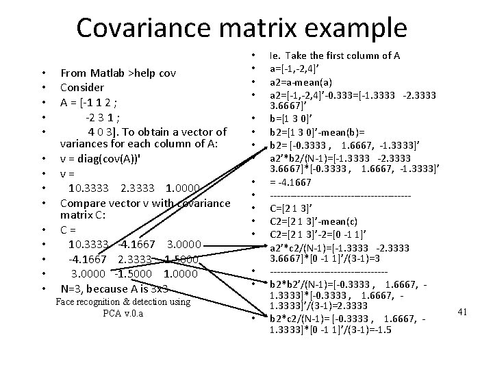
Covariance matrix example • • • • From Matlab >help cov Consider A = [-1 1 2 ; -2 3 1 ; 4 0 3]. To obtain a vector of variances for each column of A: v = diag(cov(A))' v= 10. 3333 2. 3333 1. 0000 Compare vector v with covariance matrix C: C= 10. 3333 -4. 1667 3. 0000 -4. 1667 2. 3333 -1. 5000 3. 0000 -1. 5000 1. 0000 N=3, because A is 3 x 3 Face recognition & detection using PCA v. 0. a • • • • • Ie. Take the first column of A a=[-1, -2, 4]’ a 2=a-mean(a) a 2=[-1, -2, 4]’-0. 333=[-1. 3333 -2. 3333 3. 6667]’ b=[1 3 0]’ b 2=[1 3 0]’-mean(b)= b 2= [-0. 3333 , 1. 6667, -1. 3333]’ a 2’*b 2/(N-1)=[-1. 3333 -2. 3333 3. 6667]*[-0. 3333 , 1. 6667, -1. 3333]’ = -4. 1667 ---------------------C=[2 1 3]’ C 2=[2 1 3]’-mean(c) C 2=[2 1 3]’-2=[0 -1 1]’ a 2’*c 2/(N-1)=[-1. 3333 -2. 3333 3. 6667]*[0 -1 1]’/(3 -1)=3 -----------------b 2*b 2’/(N-1)=[-0. 3333 , 1. 6667, 1. 3333]*[-0. 3333 , 1. 6667, 1. 3333]’/(3 -1)=2. 3333 b 2*c 2/(N-1)= [-0. 3333 , 1. 6667, 1. 3333]*[0 -1 1]’/(3 -1)=-1. 5 41

Mathematical methods in Statistics 3. Eigen value and Eigen vector Face recognition & detection using PCA v. 0. a 42

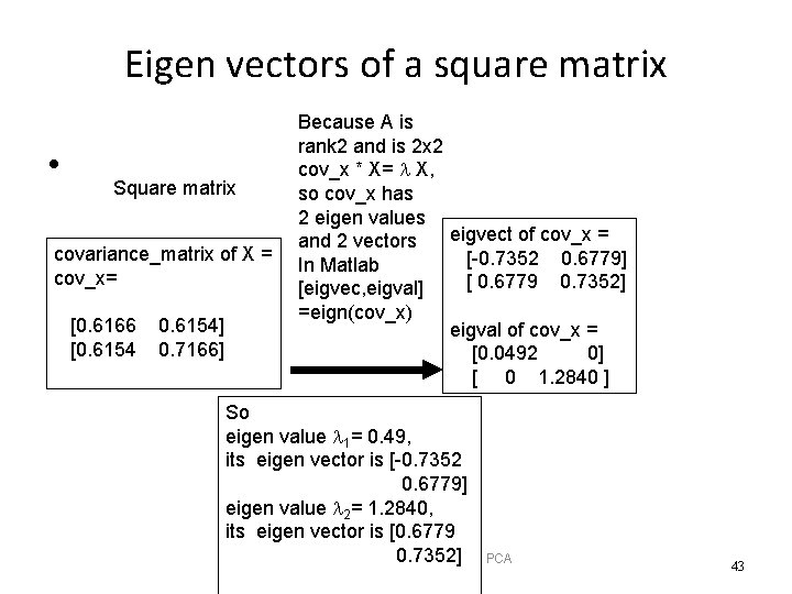
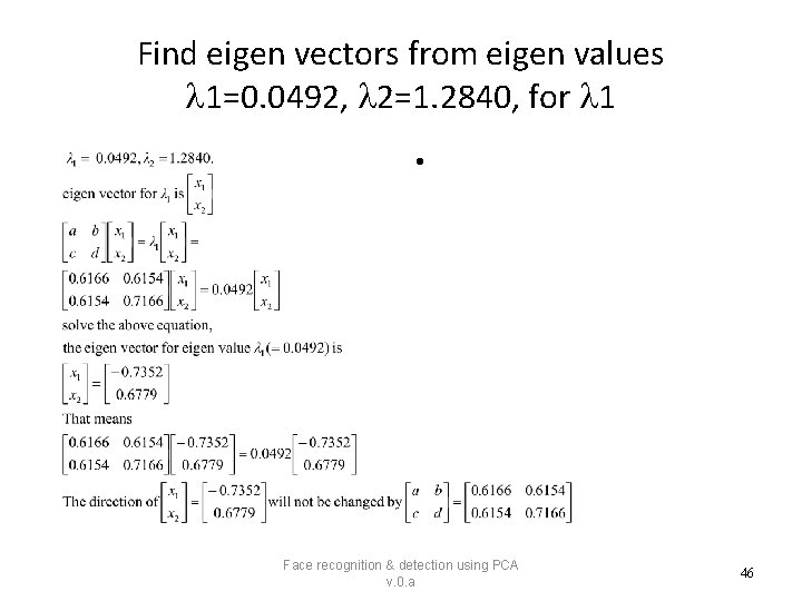
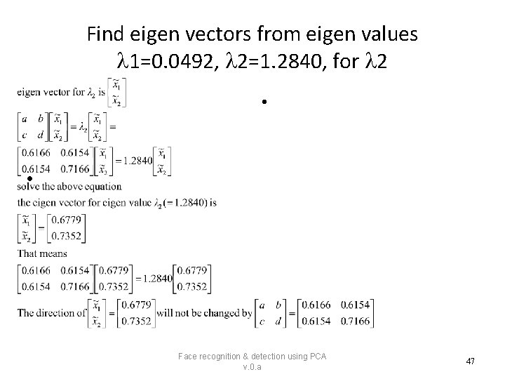
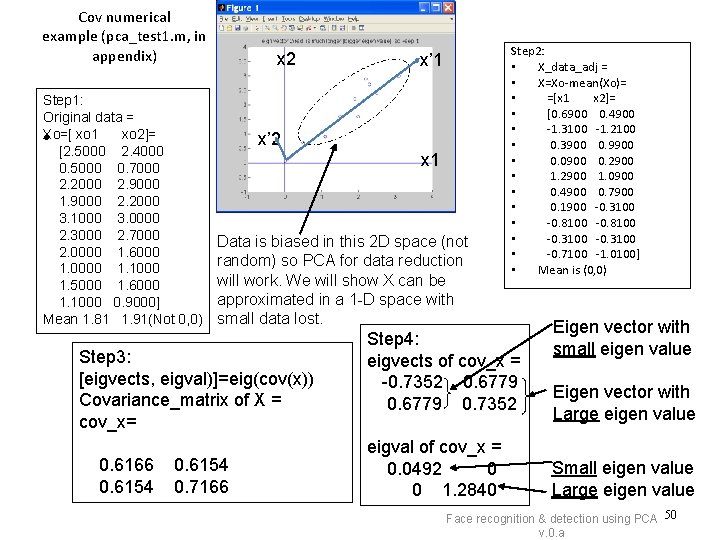
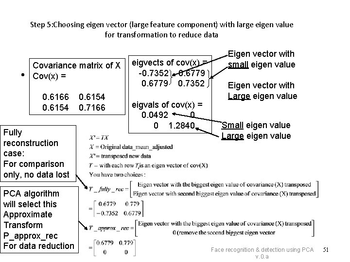
Eigen vectors of a square matrix • Square matrix covariance_matrix of X = cov_x= [0. 6166 [0. 6154] 0. 7166] Because A is rank 2 and is 2 x 2 cov_x * X= X, so cov_x has 2 eigen values eigvect of cov_x = and 2 vectors [-0. 7352 0. 6779] In Matlab [ 0. 6779 0. 7352] [eigvec, eigval] =eign(cov_x) eigval of cov_x = [0. 0492 0] [ 0 1. 2840 ] So eigen value 1= 0. 49, its eigen vector is [-0. 7352 0. 6779] eigen value 2= 1. 2840, its eigen vector is [0. 6779 0. 7352] Face recognition & detection using PCA v. 0. a 43

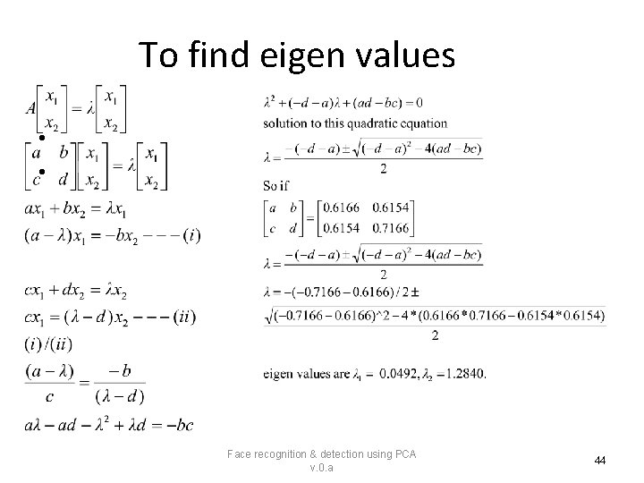
To find eigen values • • Face recognition & detection using PCA v. 0. a 44

What is an Eigen vector? AX= X (by definition) A=[a b c d] is the Eigen value and is a scalar. X=[x 1 x 2] The direction of Eigen vectors of A will not be changed by transformation A. • If A is 2 by 2, there are 2 Eigen values and 2 vectors. • • Face recognition & detection using PCA v. 0. a 45

Find eigen vectors from eigen values 1=0. 0492, 2=1. 2840, for 1 • Face recognition & detection using PCA v. 0. a 46

Find eigen vectors from eigen values 1=0. 0492, 2=1. 2840, for 2 • • Face recognition & detection using PCA v. 0. a 47

Eigen vectors of a square matrix, example 2 • Example when A is 3 x 3 • To be added, we should have 3 Eigen values and 3 Eigen vectors Face recognition & detection using PCA v. 0. a 48

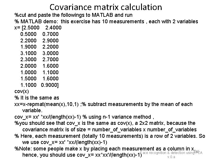
Covariance matrix calculation %cut and paste the followings to MATLAB and run % MATLAB demo: this exercise has 10 measurements , each with 2 variables x= [2. 5000 2. 4000 0. 5000 0. 7000 2. 2000 2. 9000 1. 9000 2. 2000 3. 1000 3. 0000 2. 3000 2. 7000 2. 0000 1. 6000 1. 0000 1. 1000 1. 5000 1. 6000 1. 1000 0. 9000] cov(x) % It is the same as xx=x-repmat(mean(x), 10, 1) ; % subtract measurements by the mean of each variable. cov_x= xx' *xx/(length(xx)-1) % using n-1 variance method , %you should see that cov_x is the same as cov(x), a 2 x 2 matrix, because the covariance matrix is of size = number_of_variables x number_of_variables % Here, each measurement (totally 10 measurements) is a row of 2 variables. So we use cov_x= xx' *xx/(length(xx)-1) %Note: some people make x by placing each measurement as a column in x, a 49 Face recognition & detection using PCA hence, you should use cov_x= xx*xx'/(length(xx)-1) v. 0. a

Cov numerical example (pca_test 1. m, in appendix) Step 1: Original data = Xo=[ • xo 1 xo 2]= [2. 5000 2. 4000 0. 5000 0. 7000 2. 2000 2. 9000 1. 9000 2. 2000 3. 1000 3. 0000 2. 3000 2. 7000 2. 0000 1. 6000 1. 0000 1. 1000 1. 5000 1. 6000 1. 1000 0. 9000] Mean 1. 81 1. 91(Not 0, 0) x 2 x’ 2 x 1 Data is biased in this 2 D space (not random) so PCA for data reduction will work. We will show X can be approximated in a 1 -D space with small data lost. Step 3: [eigvects, eigval)]=eig(cov(x)) Covariance_matrix of X = cov_x= 0. 6166 0. 6154 x’ 1 0. 6154 0. 7166 Step 2: • X_data_adj = • X=Xo-mean(Xo)= • =[x 1 x 2]= • [0. 6900 0. 4900 • -1. 3100 -1. 2100 • 0. 3900 0. 9900 • 0. 0900 0. 2900 • 1. 2900 1. 0900 • 0. 4900 0. 7900 • 0. 1900 -0. 3100 • -0. 8100 • -0. 3100 • -0. 7100 -1. 0100] • Mean is (0, 0) Step 4: eigvects of cov_x = -0. 7352 0. 6779 0. 7352 eigval of cov_x = 0. 0492 0 0 1. 2840 Eigen vector with small eigen value Eigen vector with Large eigen value Small eigen value Large eigen value Face recognition & detection using PCA 50 v. 0. a

Step 5: Choosing eigen vector (large feature component) with large eigen value for transformation to reduce data • Covariance matrix of X Cov(x) = 0. 6166 0. 6154 Fully reconstruction case: For comparison only, no data lost PCA algorithm will select this Approximate Transform P_approx_rec For data reduction 0. 6154 0. 7166 eigvects of cov(x) = -0. 7352 0. 6779 0. 7352 eigvals of cov(x) = 0. 0492 0 0 1. 2840 Eigen vector with small eigen value Eigen vector with Large eigen value Small eigen value Large eigen value Face recognition & detection using PCA v. 0. a 51

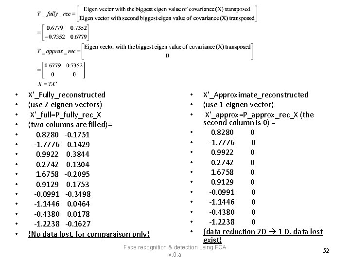
• • • • X’_Fully_reconstructed (use 2 eignen vectors) X’_full=P_fully_rec_X (two columns are filled)= 0. 8280 -0. 1751 -1. 7776 0. 1429 0. 9922 0. 3844 0. 2742 0. 1304 1. 6758 -0. 2095 0. 9129 0. 1753 -0. 0991 -0. 3498 -1. 1446 0. 0464 -0. 4380 0. 0178 -1. 2238 -0. 1627 {No data lost, for comparaison only} • • • • X’_Approximate_reconstructed (use 1 eignen vector) X’_approx=P_approx_rec_X (the second column is 0) = 0. 8280 0 -1. 7776 0 0. 9922 0 0. 2742 0 1. 6758 0 0. 9129 0 -0. 0991 0 -1. 1446 0 -0. 4380 0 -1. 2238 0 {data reduction 2 D 1 D, data lost exist} Face recognition & detection using PCA v. 0. a 52

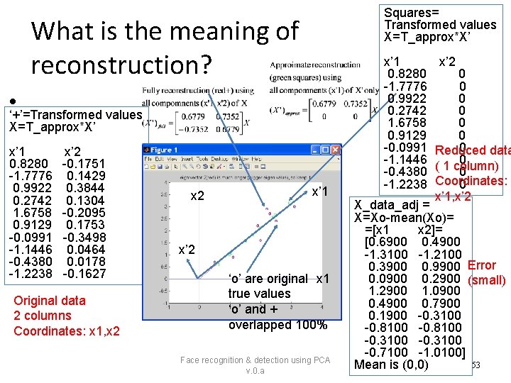
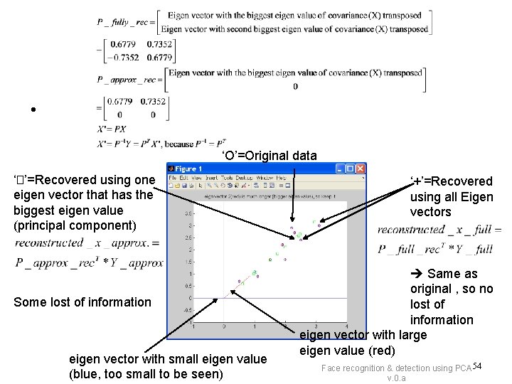
Squares= Transformed values X=T_approx*X’ What is the meaning of reconstruction? • ‘+’=Transformed values X=T_approx*X’ x’ 1 0. 8280 -1. 7776 0. 9922 0. 2742 1. 6758 0. 9129 -0. 0991 -1. 1446 -0. 4380 -1. 2238 x’ 2 -0. 1751 0. 1429 0. 3844 0. 1304 -0. 2095 0. 1753 -0. 3498 0. 0464 0. 0178 -0. 1627 Original data 2 columns Coordinates: x 1, x 2 x’ 1 x’ 2 ‘o’ are original x 1 true values ‘o’ and + overlapped 100% Face recognition & detection using PCA v. 0. a x’ 1 0. 8280 -1. 7776 0. 9922 0. 2742 1. 6758 0. 9129 -0. 0991 -1. 1446 -0. 4380 -1. 2238 x’ 2 0 0 0 0 Reduced data 0 ( 1 column) 0 Coordinates: 0 x’ 1, x’ 2 X_data_adj = X=Xo-mean(Xo)= =[x 1 x 2]= [0. 6900 0. 4900 -1. 3100 -1. 2100 0. 3900 0. 9900 Error 0. 0900 0. 2900 (small) 1. 2900 1. 0900 0. 4900 0. 7900 0. 1900 -0. 3100 -0. 8100 -0. 3100 -0. 7100 -1. 0100] 53 Mean is (0, 0)

• ‘O’=Original data ‘�’=Recovered using one eigen vector that has the biggest eigen value (principal component) Some lost of information eigen vector with small eigen value (blue, too small to be seen) ‘+’=Recovered using all Eigen vectors Same as original , so no lost of information eigen vector with large eigen value (red) Face recognition & detection using PCA 54 v. 0. a

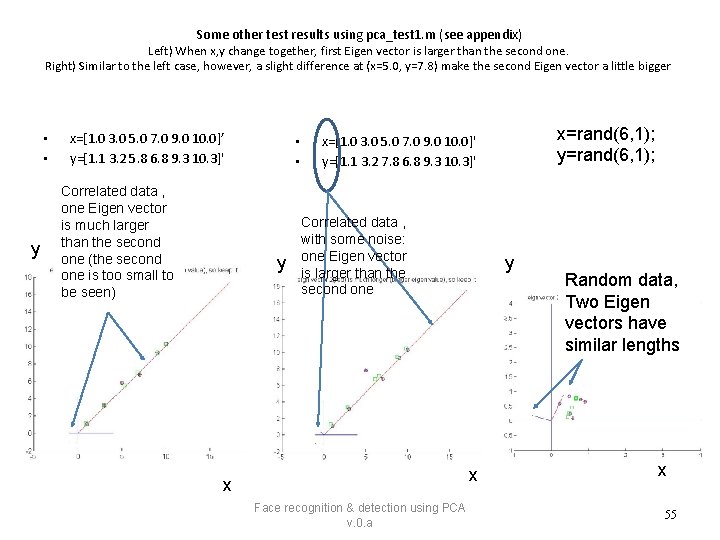
Some other test results using pca_test 1. m (see appendix) Left) When x, y change together, first Eigen vector is larger than the second one. Right) Similar to the left case, however, a slight difference at (x=5. 0, y=7. 8) make the second Eigen vector a little bigger • • y x=[1. 0 3. 0 5. 0 7. 0 9. 0 10. 0]’ y=[1. 1 3. 2 5. 8 6. 8 9. 3 10. 3]' Correlated data , one Eigen vector is much larger than the second one (the second one is too small to be seen) • • y x=rand(6, 1); y=rand(6, 1); x=[1. 0 3. 0 5. 0 7. 0 9. 0 10. 0]' y=[1. 1 3. 2 7. 8 6. 8 9. 3 10. 3]' Correlated data , with some noise: one Eigen vector is larger than the second one y x x Face recognition & detection using PCA v. 0. a Random data, Two Eigen vectors have similar lengths x 55

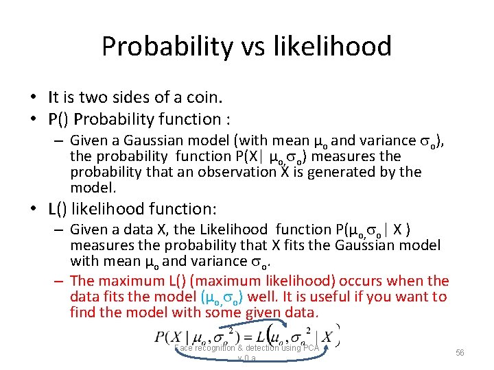
Probability vs likelihood • It is two sides of a coin. • P() Probability function : – Given a Gaussian model (with mean µo and variance o), the probability function P(X| µo, o) measures the probability that an observation X is generated by the model. • L() likelihood function: – Given a data X, the Likelihood function P(µo, o| X ) measures the probability that X fits the Gaussian model with mean µo and variance o. – The maximum L() (maximum likelihood) occurs when the data fits the model (µo, o) well. It is useful if you want to find the model with some given data. Face recognition & detection using PCA v. 0. a 56

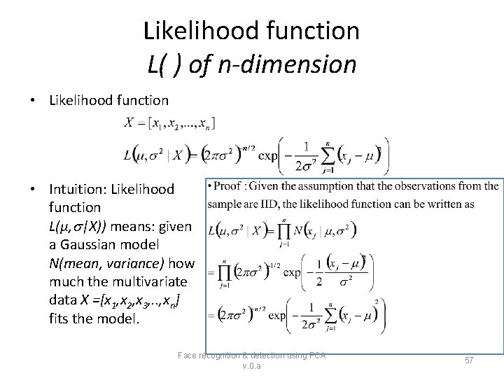
Likelihood function L( ) of n-dimension • Likelihood function • Intuition: Likelihood function L(µ, |X)) means: given a Gaussian model N(mean, variance) how much the multivariate data X =[x 1, x 2, x 3, . . , xn] fits the model. Face recognition & detection using PCA v. 0. a 57

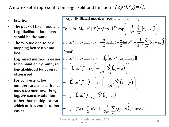
A more useful representation Log-Likelihood function= Log(L( • • • ))=l () Intuition: The peak of Likelihood and Log-Likelihood functions should be the same. The two are one to one mapping hence no data loss. Log based method is easier to be handled by math, so log-Likelihood function is often used For computers, log numbers are smaller hence may save memory. Using log, we can use addition rather than multiplication which makes computation easier. Face recognition & detection using PCA v. 0. a 58

Exercise 3: Maximum Log-Likelihood function Face recognition & detection using PCA https: //towardsdatascience. com/probability-concepts-explained-maximum-likelihood-estimation-c 7 b 4342 fdbb 1 v. 0. a 59

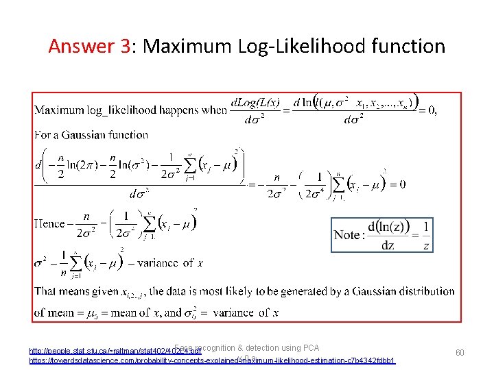
Answer 3: Maximum Log-Likelihood function Face recognition & detection using PCA http: //people. stat. sfu. ca/~raltman/stat 402/402 L 4. pdf v. 0. a https: //towardsdatascience. com/probability-concepts-explained-maximum-likelihood-estimation-c 7 b 4342 fdbb 1 60

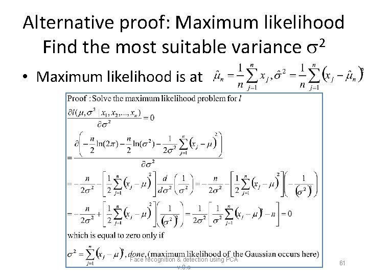
Alternative proof: Maximum likelihood Find the most suitable variance 2 • Maximum likelihood is at Face recognition & detection using PCA v. 0. a 61

Linear Algebra (draft) https: //en. wikipedia. org/wiki/Kernel_(linear_algebra ) KH Wong Face recognition & detection using PCA v. 0. a 62

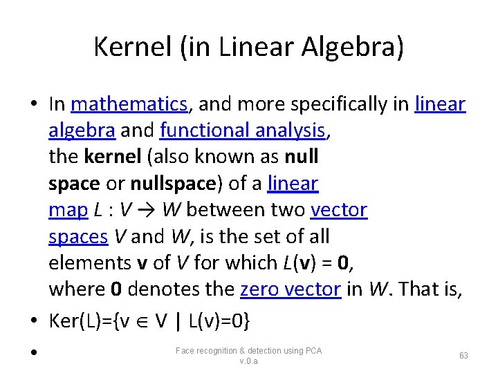
Kernel (in Linear Algebra) • In mathematics, and more specifically in linear algebra and functional analysis, the kernel (also known as null space or nullspace) of a linear map L : V → W between two vector spaces V and W, is the set of all elements v of V for which L(v) = 0, where 0 denotes the zero vector in W. That is, • Ker(L)={v V | L(v)=0} • Face recognition & detection using PCA v. 0. a 63

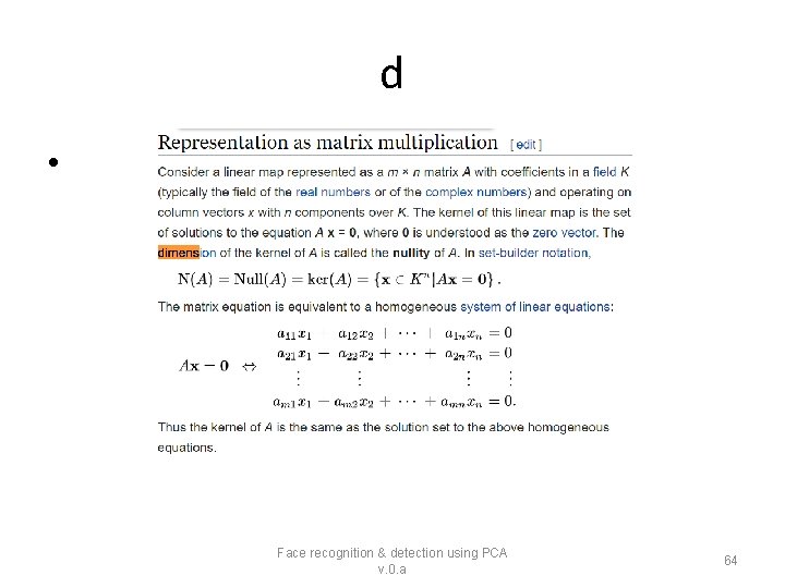
d • Face recognition & detection using PCA v. 0. a 64

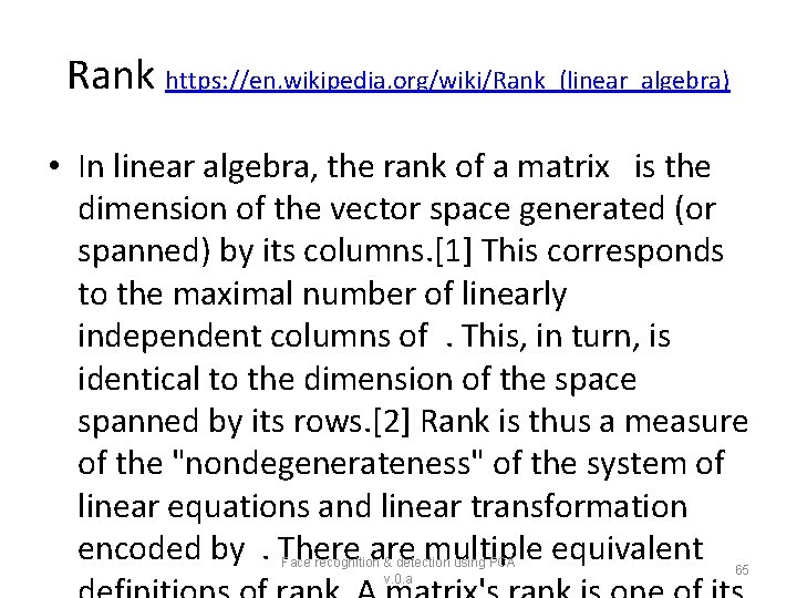
Rank https: //en. wikipedia. org/wiki/Rank_(linear_algebra) • In linear algebra, the rank of a matrix is the dimension of the vector space generated (or spanned) by its columns. [1] This corresponds to the maximal number of linearly independent columns of. This, in turn, is identical to the dimension of the space spanned by its rows. [2] Rank is thus a measure of the "nondegenerateness" of the system of linear equations and linear transformation encoded by. There are multiple equivalent Face recognition & detection using PCA v. 0. a 65

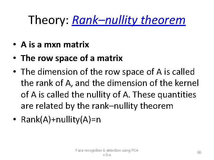
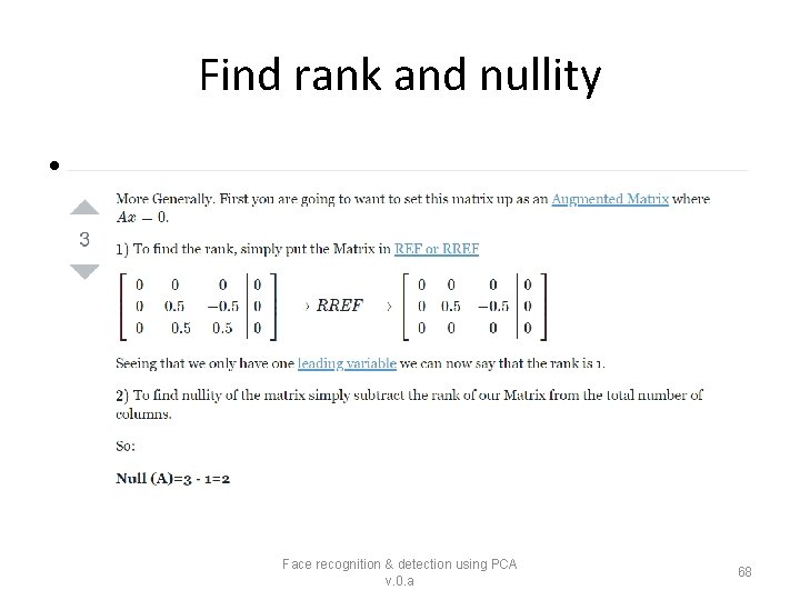
Theory: Rank–nullity theorem • A is a mxn matrix • The row space of a matrix • The dimension of the row space of A is called the rank of A, and the dimension of the kernel of A is called the nullity of A. These quantities are related by the rank–nullity theorem • Rank(A)+nullity(A)=n Face recognition & detection using PCA v. 0. a 66

Left null space Face recognition & detection using PCA v. 0. a 67

Find rank and nullity • Face recognition & detection using PCA v. 0. a 68

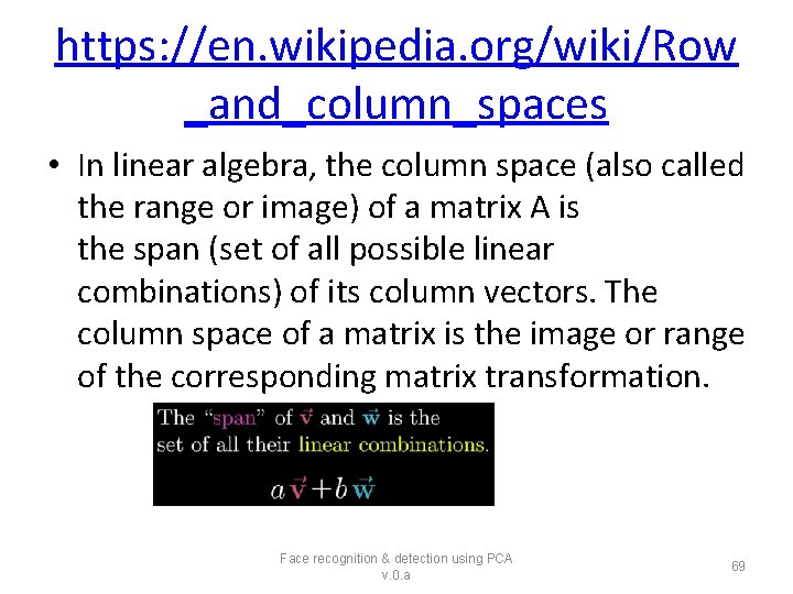
https: //en. wikipedia. org/wiki/Row _and_column_spaces • In linear algebra, the column space (also called the range or image) of a matrix A is the span (set of all possible linear combinations) of its column vectors. The column space of a matrix is the image or range of the corresponding matrix transformation. Face recognition & detection using PCA v. 0. a 69

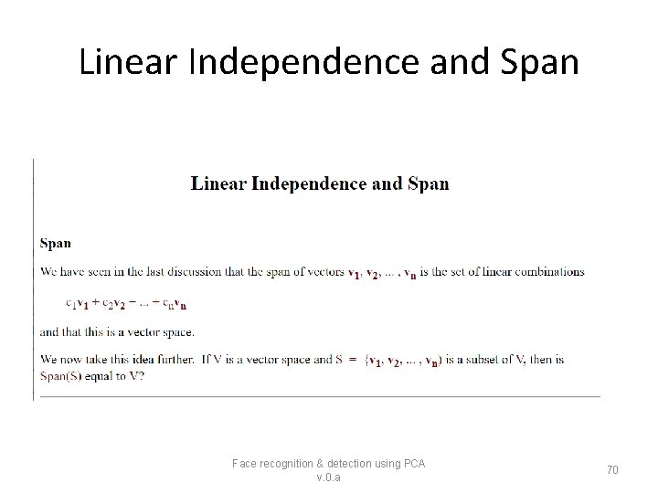
Linear Independence and Span Face recognition & detection using PCA v. 0. a 70