Computer Vision Sampling and Quantisation Computer Vision Sampling

Computer Vision Sampling and Quantisation

Computer Vision Sampling & quantisation o 1. Discretization of continuous signals o 2. Signal representation in the spatial and frequency domain o 3. Effects of sampling and quantisation o 4. More on sampling o 5. More on quantisation

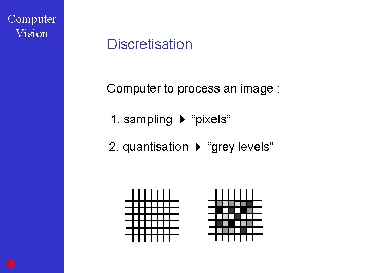
Computer Vision Discretisation Computer to process an image : 1. sampling 4 “pixels” 2. quantisation 4 “grey levels”

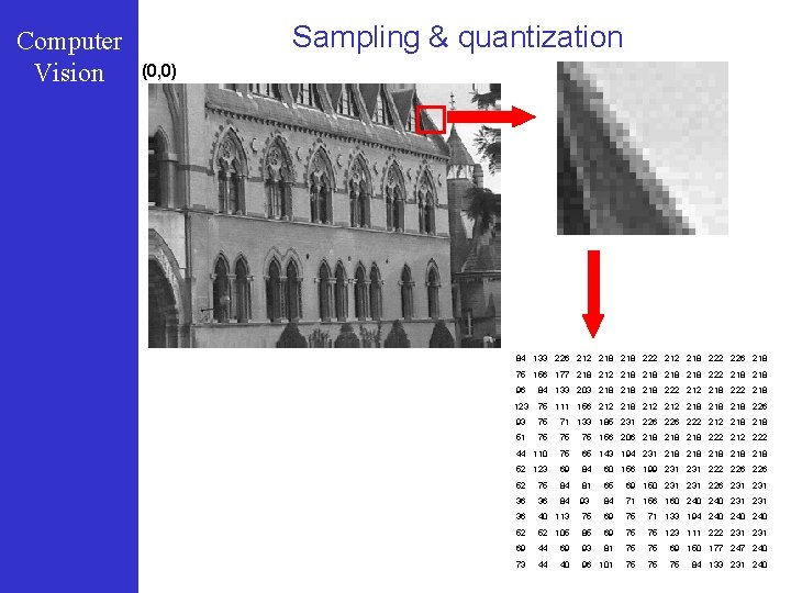
Computer Vision Sampling & quantization (0, 0) 84 133 226 212 218 222 226 218 75 156 177 218 212 218 218 222 218 96 84 133 203 218 218 222 218 123 75 111 156 212 218 218 226 93 75 71 133 185 231 226 222 218 218 51 75 75 75 156 206 218 218 222 212 222 44 110 75 65 143 194 231 218 218 218 52 123 69 84 60 156 199 231 222 226 52 75 84 81 65 69 150 231 226 231 36 36 84 93 84 71 156 160 240 231 36 40 113 75 69 75 71 133 194 240 240 52 52 105 85 69 75 75 123 111 222 231 69 44 69 93 81 75 75 69 150 177 240 73 44 40 96 101 75 75 75 84 133 231 240

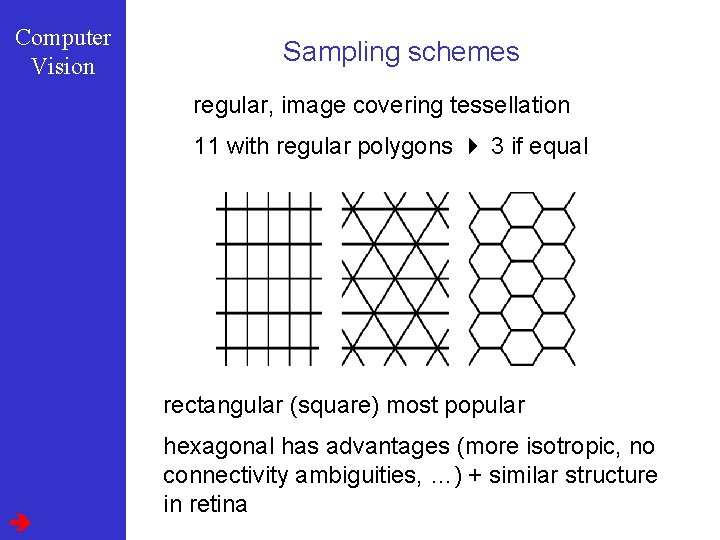
Computer Vision Sampling schemes regular, image covering tessellation 11 with regular polygons 4 3 if equal rectangular (square) most popular hexagonal has advantages (more isotropic, no connectivity ambiguities, …) + similar structure in retina

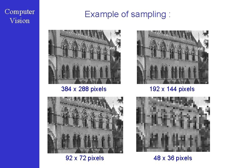
Computer Vision Example of sampling : 384 x 288 pixels 192 x 144 pixels 92 x 72 pixels 48 x 36 pixels

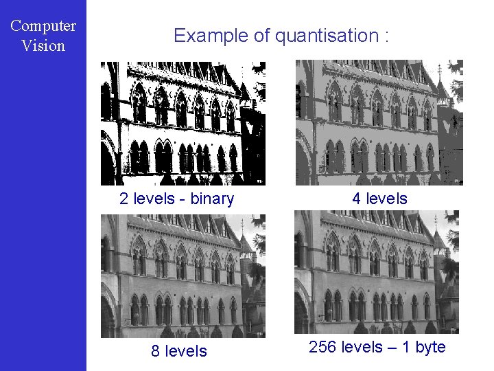
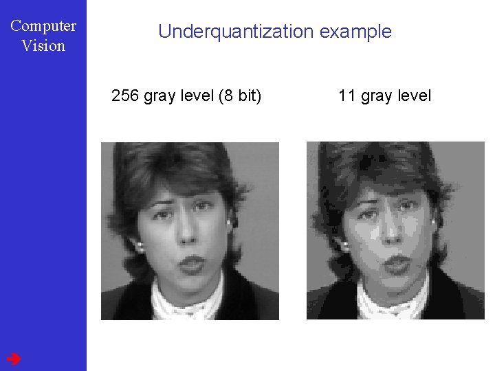
Computer Vision Example of quantisation : 2 levels - binary 4 levels 8 levels 256 levels – 1 byte

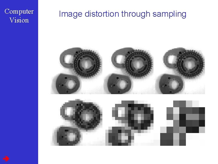
Computer Vision Image distortion through sampling

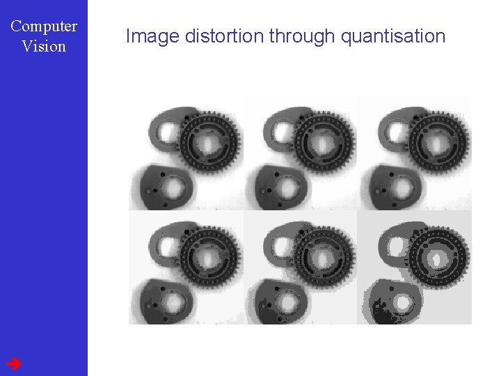
Computer Vision Image distortion through quantisation

Computer Vision Remarks o 1. Importance of binary images o 2. Non-uniform sampling and/or quantisation n a. fine sampling for details n b. fine quantisation for homogeneous regions

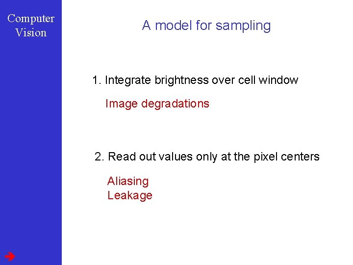
Computer Vision A model for sampling 1. Integrate brightness over cell window Image degradations 2. Read out values only at the pixel centers Aliasing Leakage

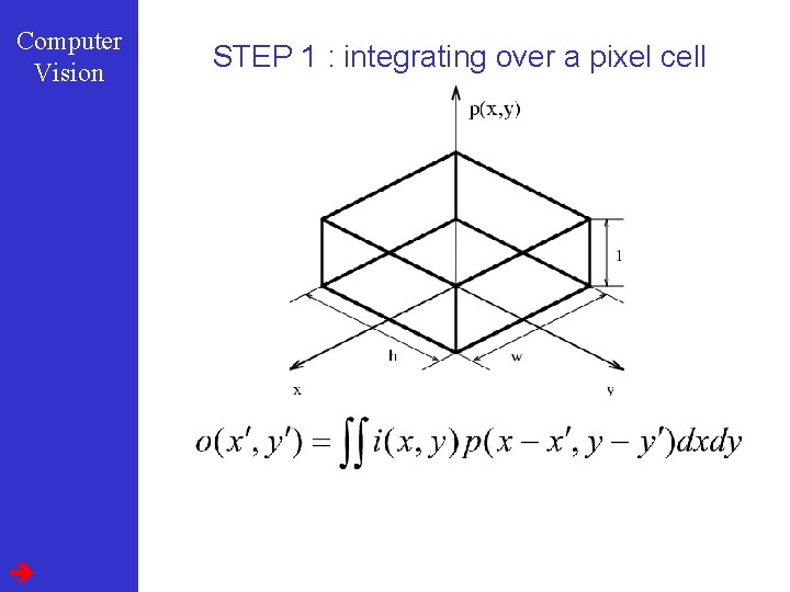
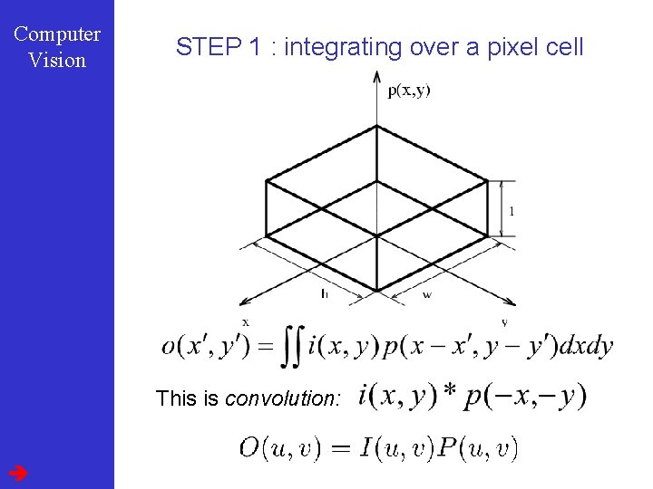
Computer Vision STEP 1 : integrating over a pixel cell

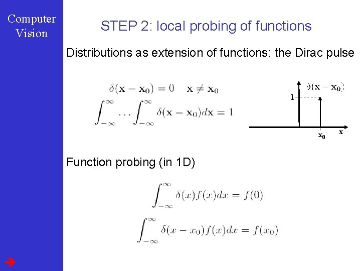
Computer Vision STEP 2: local probing of functions Distributions as extension of functions: the Dirac pulse 1 x 0 Function probing (in 1 D) x

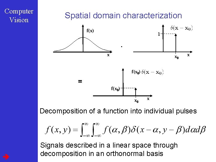
Computer Vision Spatial domain characterization f(x) 1 . x x 0 x f(x 0) = f(x 0) x 0 x Decomposition of a function into individual pulses Signals described in a linear space through decomposition in an orthonormal basis

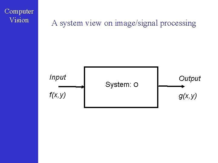
Computer Vision A system view on image/signal processing Input f(x, y) System: O Output g(x, y)

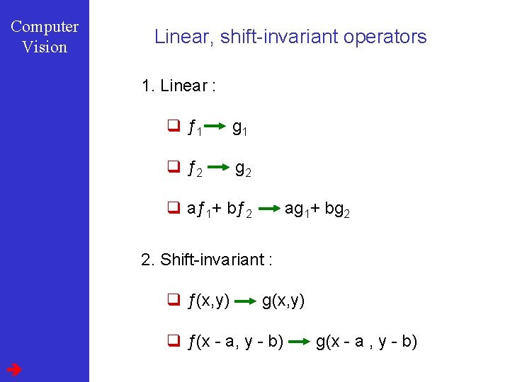
Computer Vision Linear, shift-invariant operators 1. Linear : q ƒ 1 g 1 q ƒ 2 g 2 q aƒ 1+ bƒ 2 ag 1+ bg 2 2. Shift-invariant : q ƒ(x, y) g(x, y) q ƒ(x - a, y - b) g(x - a , y - b)

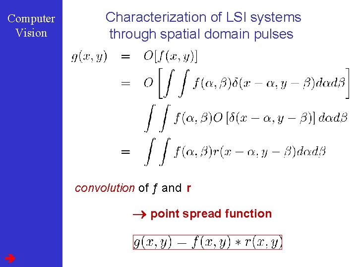
Computer Vision Characterization of LSI systems through spatial domain pulses convolution of ƒ and hr point spread function

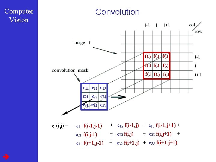
Computer Vision Convolution f(. ) f(. ) c 11 c 12 c 13 c 21 c 22 c 23 c 31 c 32 c 33 o (i, j) = c 11 f(i-1, j-1) + c 12 f(i-1, j) + c 13 f(i-1, j+1) + c 21 f(i, j-1) + c 22 f(i, j) c 31 f(i+1, j-1) + c 32 f(i+1, j) + c 33 f(i+1, j+1) + c 23 f(i, j+1) +

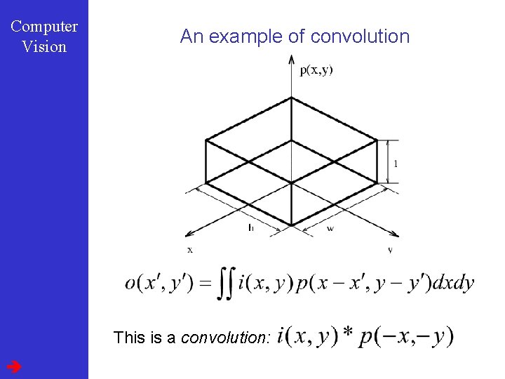
Computer Vision An example of convolution This is a convolution:

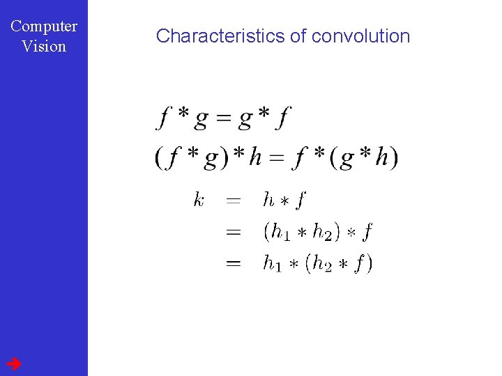
Computer Vision Characteristics of convolution

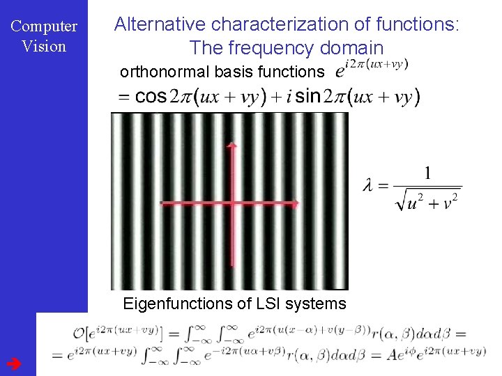
Computer Vision Alternative characterization of functions: The frequency domain orthonormal basis functions Eigenfunctions of LSI systems

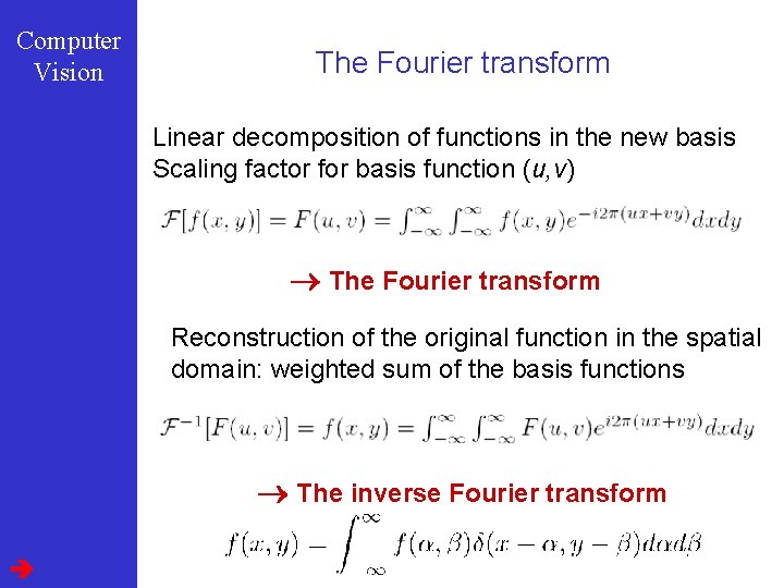
Computer Vision The Fourier transform Linear decomposition of functions in the new basis Scaling factor for basis function (u, v) The Fourier transform Reconstruction of the original function in the spatial domain: weighted sum of the basis functions The inverse Fourier transform

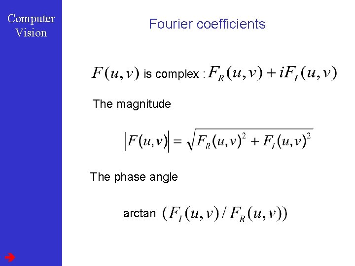
Computer Vision Fourier coefficients is complex : The magnitude The phase angle arctan

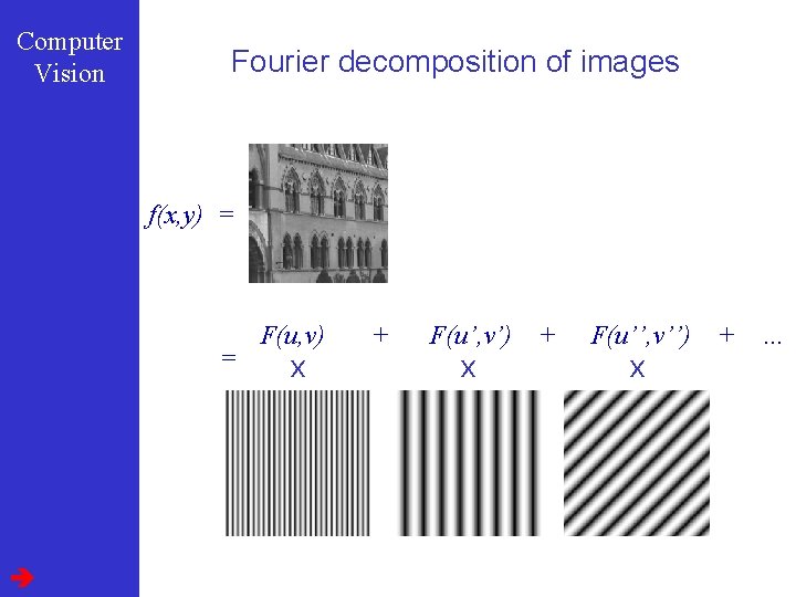
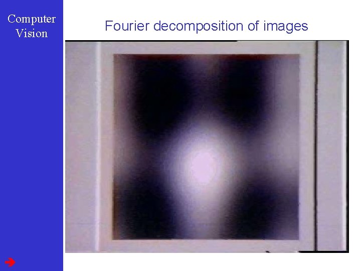
Computer Vision Fourier decomposition of images f(x, y) = = F(u, v) x + F(u’, v’) x + F(u’’, v’’) x + …

Computer Vision Fourier decomposition of images

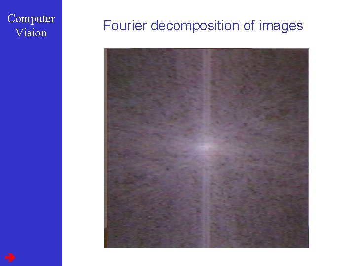
Computer Vision Fourier decomposition of images

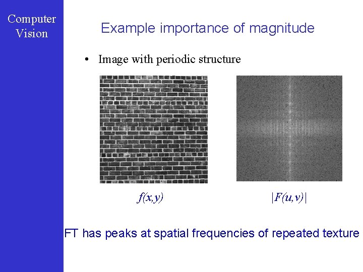
Computer Vision Example importance of magnitude • Image with periodic structure f(x, y) |F(u, v)| FT has peaks at spatial frequencies of repeated texture

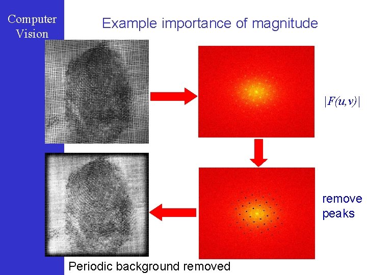
Computer Vision Example importance of magnitude |F(u, v)| remove peaks Periodic background removed

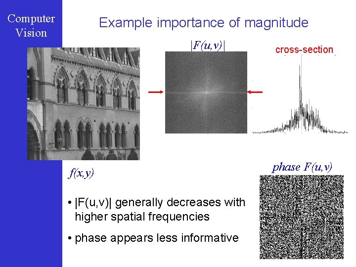
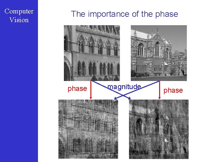
Computer Vision Example importance of magnitude |F(u, v)| f(x, y) • |F(u, v)| generally decreases with higher spatial frequencies • phase appears less informative cross-section phase F(u, v)

Computer Vision The importance of the phase magnitude phase

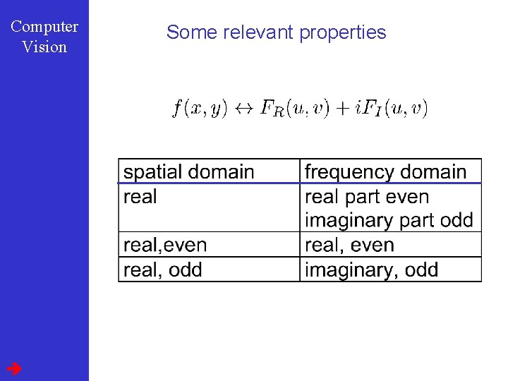
Computer Vision Some relevant properties

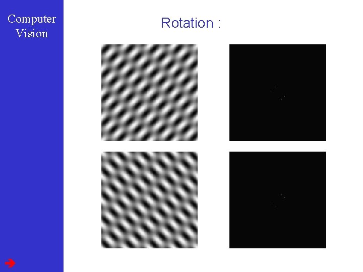
Computer Vision Rotation :

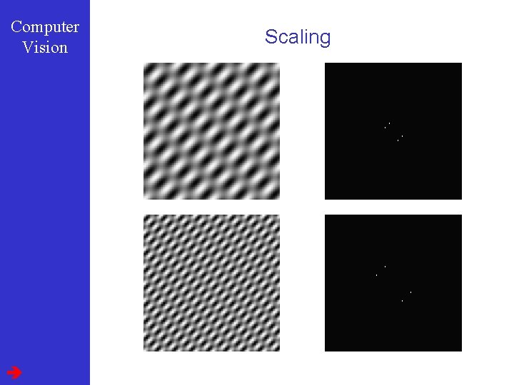
Computer Vision Scaling :

Computer Vision Affine

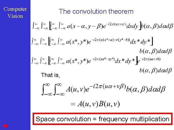
Computer Vision The convolution theorem Fourier

Computer Vision The convolution theorem That is, Space convolution = frequency multiplication

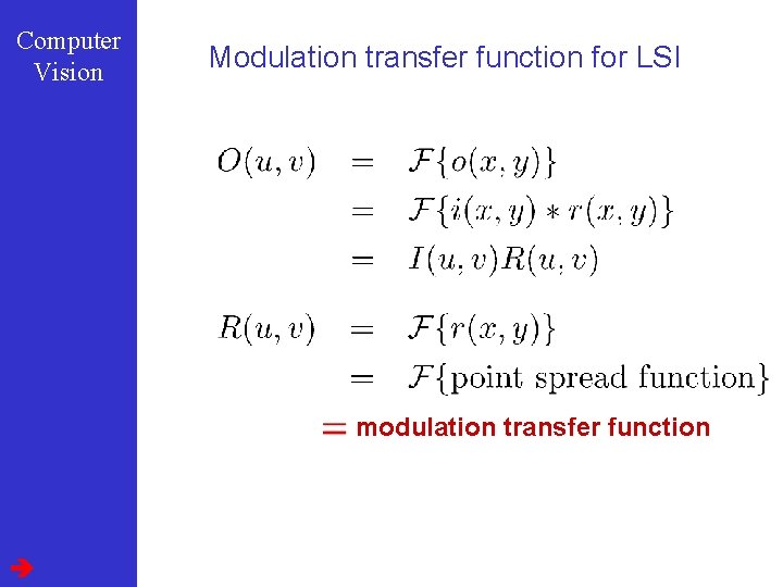
Computer Vision Modulation transfer function for LSI modulation transfer function

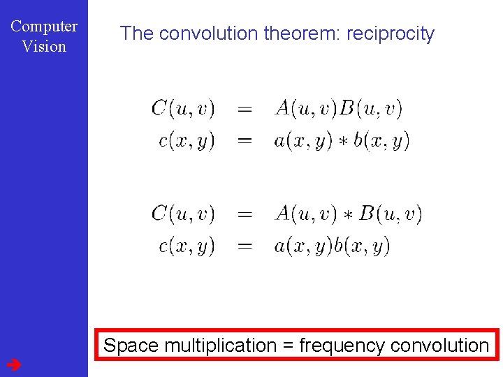
Computer Vision The convolution theorem: reciprocity Space multiplication = frequency convolution

Computer Vision A model for sampling … back to STEP 1 1. Integrate brightness over cell window Image degradations 2. Read out values only at the pixel centers Aliasing Leakage

Computer Vision STEP 1 : integrating over a pixel cell This is convolution:

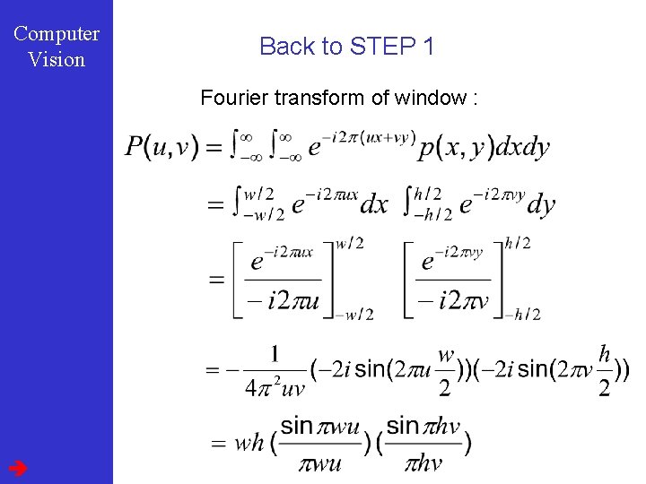
Computer Vision Back to STEP 1 Fourier transform of window :

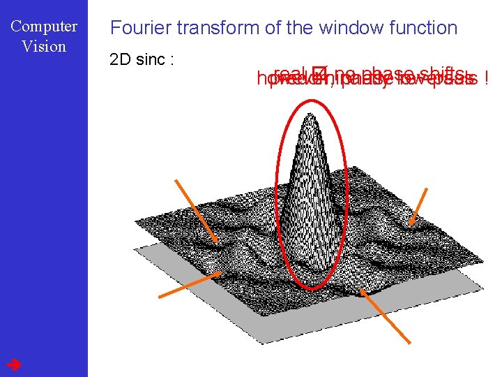
Computer Vision Fourier transform of the window function 2 D sinc : real no phase shifts ! however, predominantly phase low-pass reversals

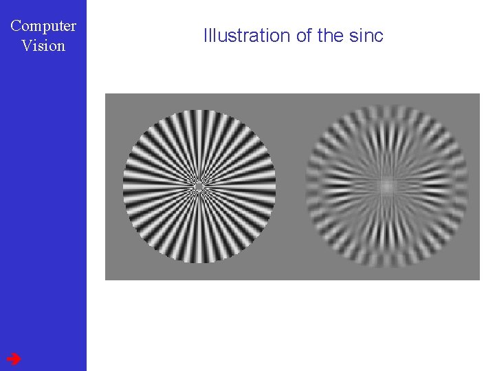
Computer Vision Illustration of the sinc

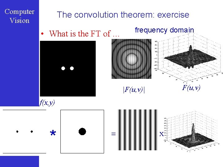
Computer Vision The convolution theorem: exercise • What is the FT of … frequency domain F(u, v) |F(u, v)| f(x, y) * = x

Computer Vision A model for sampling … back to STEP 2 1. Integrate brightness over cell window Image degradations 2. Read out values only at the pixel centers Aliasing Leakage

Computer Vision STEP 2 : discrete representation of functions In the spatial and frequency domain a) Discretizing in the spatial domain b) Limiting the spatial extent c) Discretizing in the frequency domain

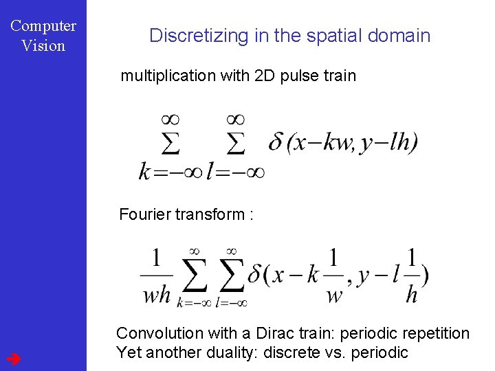
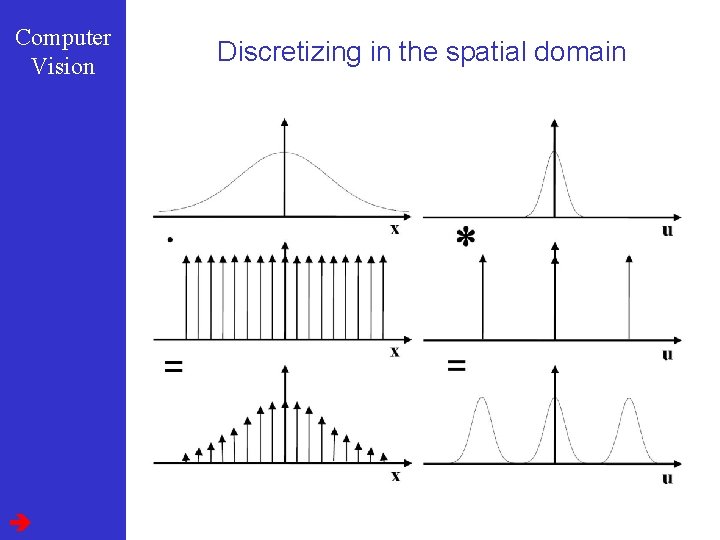
Computer Vision Discretizing in the spatial domain multiplication with 2 D pulse train Fourier transform : Convolution with a Dirac train: periodic repetition Yet another duality: discrete vs. periodic

Computer Vision Discretizing in the spatial domain

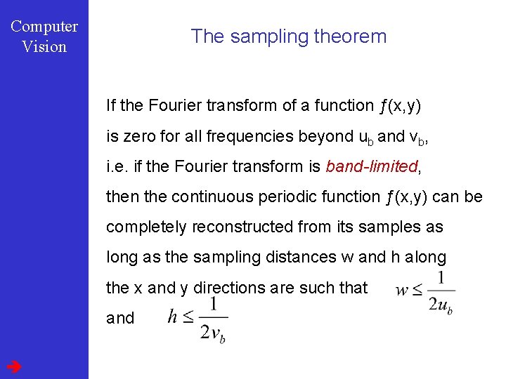
Computer Vision The sampling theorem If the Fourier transform of a function ƒ(x, y) is zero for all frequencies beyond ub and vb, i. e. if the Fourier transform is band-limited, then the continuous periodic function ƒ(x, y) can be completely reconstructed from its samples as long as the sampling distances w and h along the x and y directions are such that and

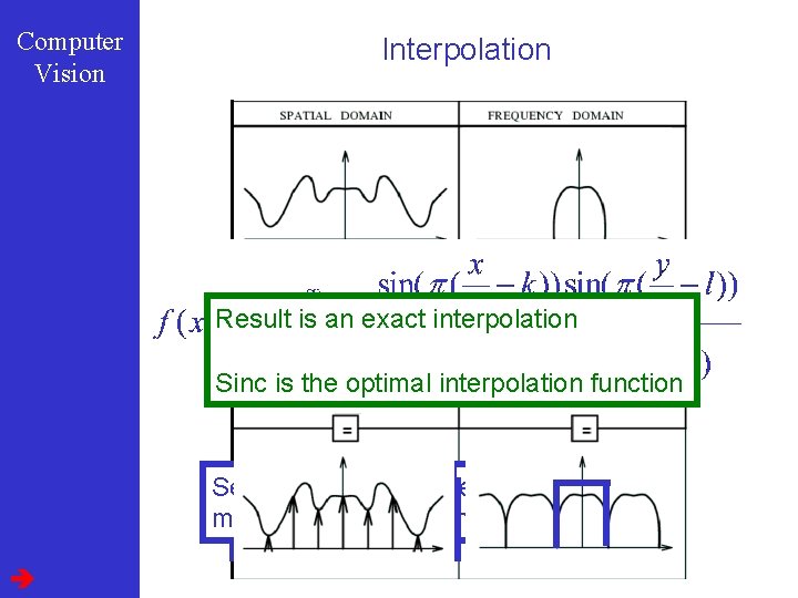
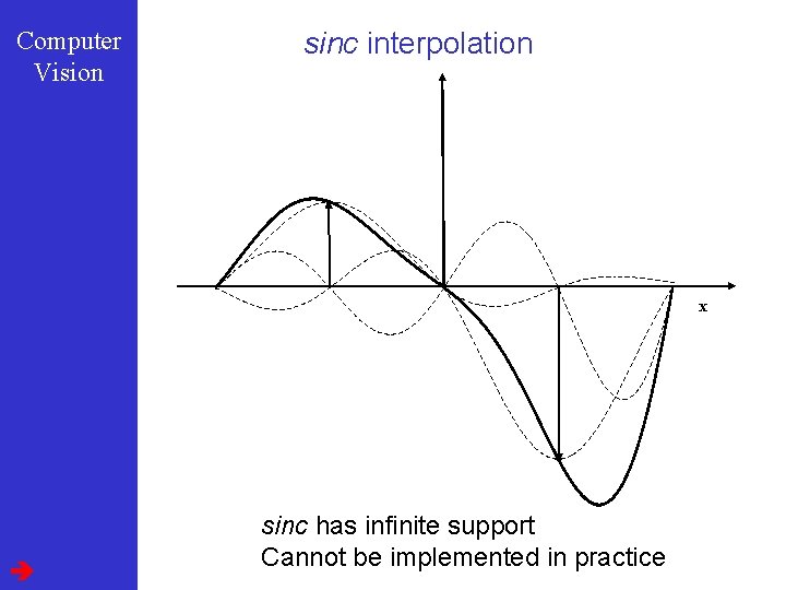
Computer Vision Interpolation Result is an exact interpolation Sample Periods must not overlap (multiply (hence Nyquist rate) Sinc is the optimal interpolation function pulse train) Select one Thus period convolve : Fourier Result is periodic multiplytransform window with pulse train Fourier transform

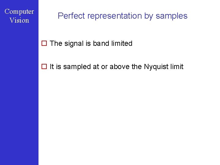
Computer Vision Perfect representation by samples o The signal is band limited o It is sampled at or above the Nyquist limit

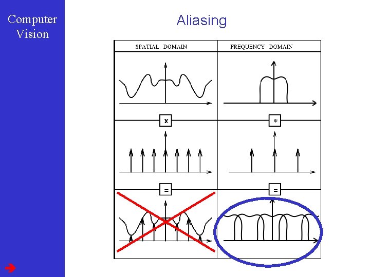
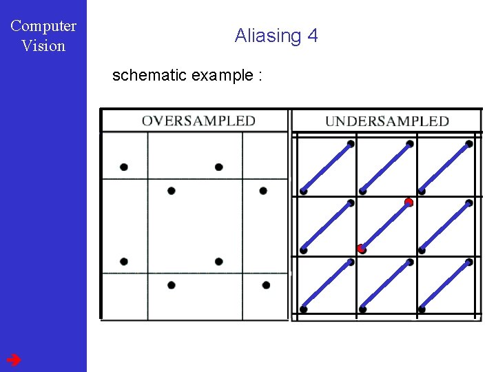
Computer Vision Aliasing

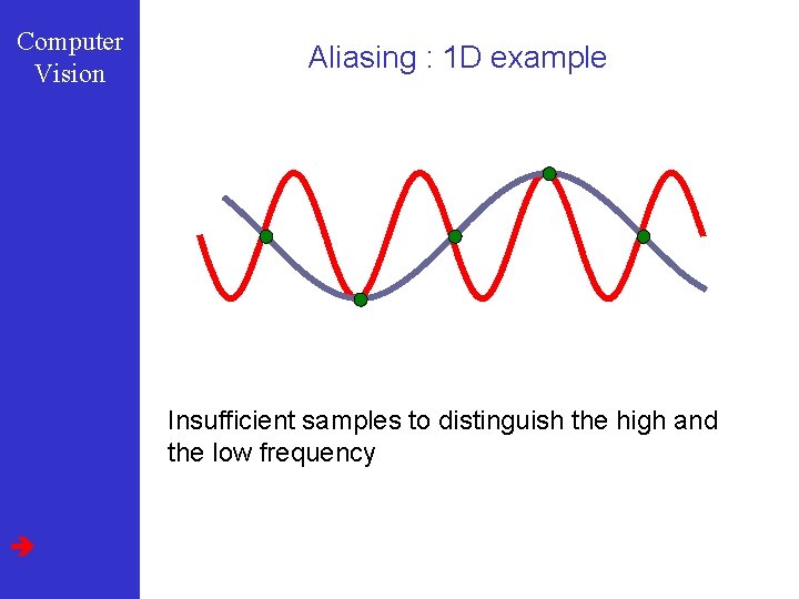
Computer Vision Aliasing : 1 D example Insufficient samples to distinguish the high and the low frequency

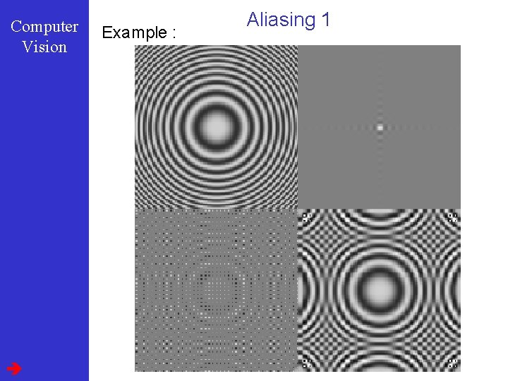
Computer Vision Example : Aliasing 1

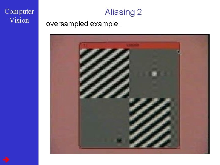
Computer Vision Aliasing 2 oversampled example :

Computer Vision Aliasing 2 oversampled example :

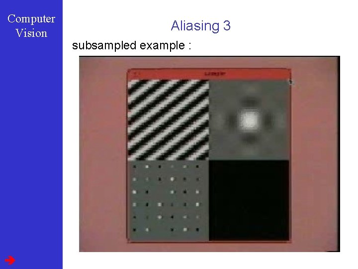
Computer Vision Aliasing 3 subsampled example :

Computer Vision Aliasing 4 schematic example :

Computer Vision sinc interpolation x sinc has infinite support Cannot be implemented in practice

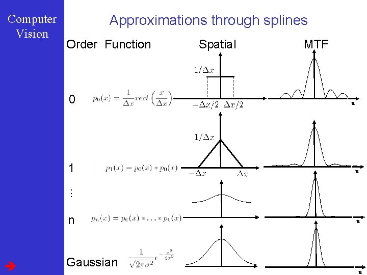
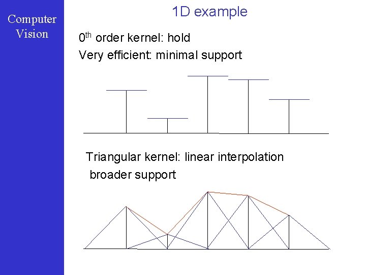
Computer Vision Approximations through splines Order Function 0 1 Spatial MTF u u . . . n Gaussian u u

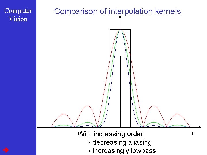
Computer Vision Comparison of interpolation kernels With increasing order • decreasing aliasing • increasingly lowpass u

Computer Vision 1 D example 0 th order kernel: hold Very efficient: minimal support Triangular kernel: linear interpolation broader support

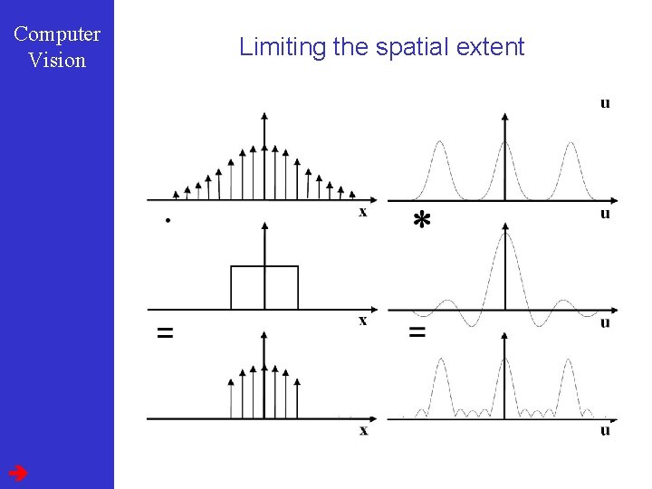
Computer Vision Limiting the spatial extent

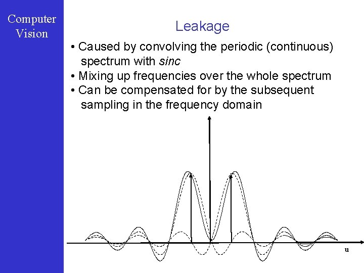
Computer Vision Leakage • Caused by convolving the periodic (continuous) spectrum with sinc • Mixing up frequencies over the whole spectrum • Can be compensated for by the subsequent sampling in the frequency domain u

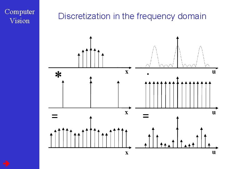
Computer Vision Discretization in the frequency domain

Computer Vision Perfect representation by samples o The signal is band limited o It is sampled at or above the Nyquist limit o The signal is periodic o Sampling is compatible with the signal period no phase difference after a finite number of periods

Computer Vision Discretization in the frequency domain

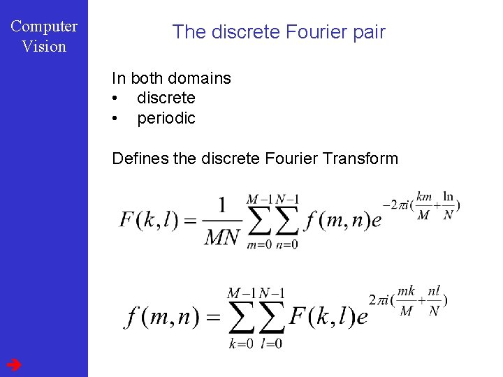
Computer Vision The discrete Fourier pair In both domains • discrete • periodic Defines the discrete Fourier Transform

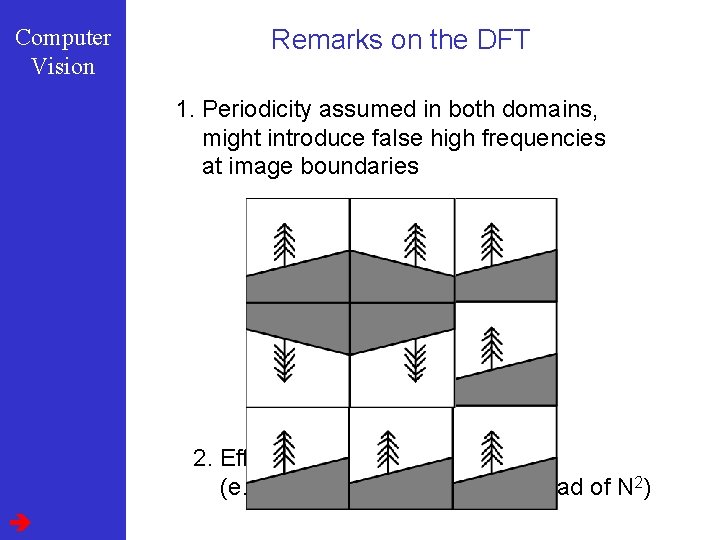
Computer Vision Remarks on the DFT 1. Periodicity assumed in both domains, might introduce false high frequencies at image boundaries 2. Efficient implementations exist (e. g. FFT which is N log 2 N instead of N 2)

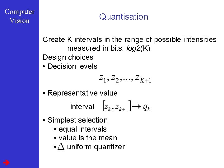
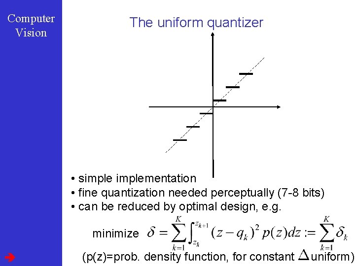
Computer Vision Quantisation Create K intervals in the range of possible intensities measured in bits: log 2(K) Design choices • Decision levels • Representative value interval • Simplest selection • equal intervals • value is the mean • uniform quantizer

Computer Vision The uniform quantizer • simplementation • fine quantization needed perceptually (7 -8 bits) • can be reduced by optimal design, e. g. minimize (p(z)=prob. density function, for constant uniform)

Computer Vision Underquantization example 256 gray level (8 bit) 11 gray level

Computer Vision Remarks • Quantization: – Often 8 bits per pixel (monochrome), 24 bits per pixel (RGB) – Medical images 12 bits (4096 levels) or 16 bits (65536 levels) • Size – Cameras typically few K width – Satellite images 2 -100 K width