Computer Vision I The Fourier Transform part 2

Computer Vision I The Fourier Transform part 2: applications Holger Heidrich 28/10/2020 Computer Vision I: Fourier Transform part 2 - applications

Roadmap this lecture part 1: theoretical background • Superposition principle • Definition, properties • Convolution • sampling theorem, connection discrete continuous, image pyramids • Fast Fourier Transform • Correlation, Autocorrelation • Regularisation • uncertainty principle part 2: applications • Fourier approximations and descriptors • Optics: Lens as F-transformer, 4 -f • Computer tomography 28/10/2020 Computer Vision I: Fourier Transform part 2 - applications 2

Literature 1. Stanford course: The Fourier Transforms and Its Applications and their course reader 2. J. F. James, A Student’s Guide to Fourier Transforms 3. Chen, Haykin, On Different Facets of Regularization Theory 4. Max Born, Emil Wolf, Principles of Optics: Electromagnetic Theory of Propagation, Interference and Diffraction of Light 5. Joseph W. Goodman, Introduction to Fourier Optics 6. Richard Szeliski, Computer Vision: Algorithms and Applications, chapt. 3+4 28/10/2020 Computer Vision I: Fourier Transform part 2 - applications 3

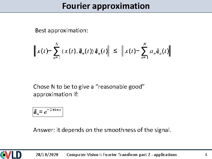
Fourier approximation Best approximation: Chose N to be to give a “reasonable good” approximation if: Answer: it depends on the smoothness of the signal. 28/10/2020 Computer Vision I: Fourier Transform part 2 - applications 4

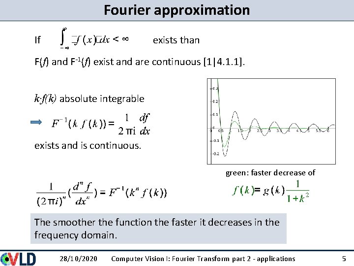
Fourier approximation If exists than F(f) and F-1(f) exist and are continuous [1|4. 1. 1]. k∙f(k) absolute integrable exists and is continuous. green: faster decrease of The smoother the function the faster it decreases in the frequency domain. 28/10/2020 Computer Vision I: Fourier Transform part 2 - applications 5

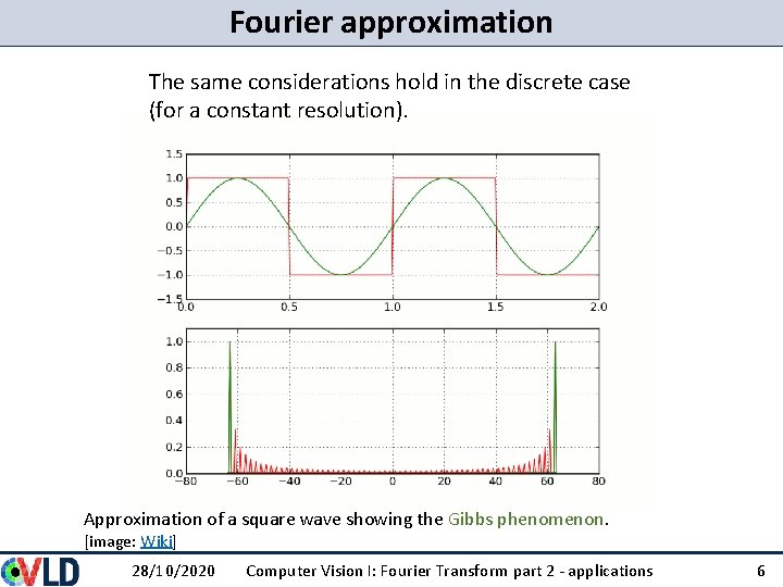
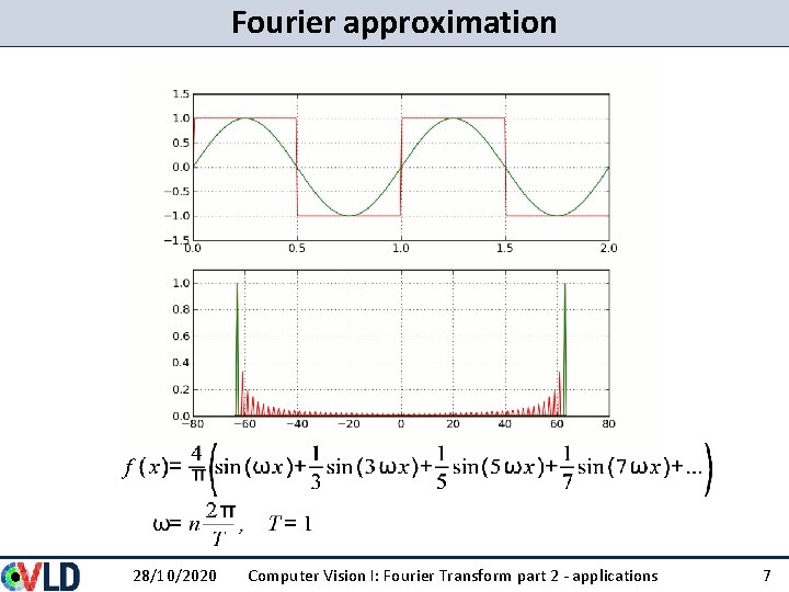
Fourier approximation The same considerations hold in the discrete case (for a constant resolution). Approximation of a square wave showing the Gibbs phenomenon. [image: Wiki] 28/10/2020 Computer Vision I: Fourier Transform part 2 - applications 6

Fourier approximation 28/10/2020 Computer Vision I: Fourier Transform part 2 - applications 7

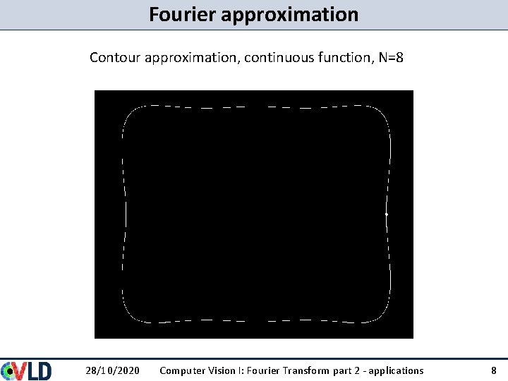
Fourier approximation Contour approximation, continuous function, N=8 28/10/2020 Computer Vision I: Fourier Transform part 2 - applications 8

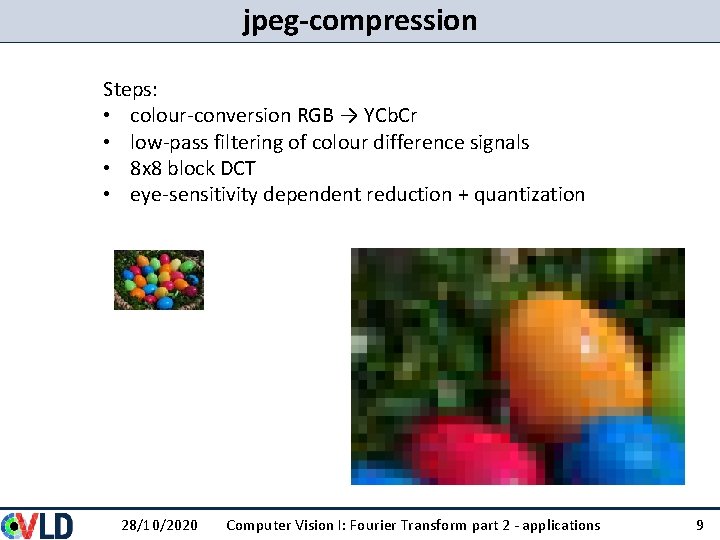
jpeg-compression Steps: • colour-conversion RGB → YCb. Cr • low-pass filtering of colour difference signals • 8 x 8 block DCT • eye-sensitivity dependent reduction + quantization 28/10/2020 Computer Vision I: Fourier Transform part 2 - applications 9

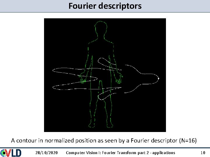
Fourier descriptors A contour in normalized position as seen by a Fourier descriptor (N=16) 28/10/2020 Computer Vision I: Fourier Transform part 2 - applications 10

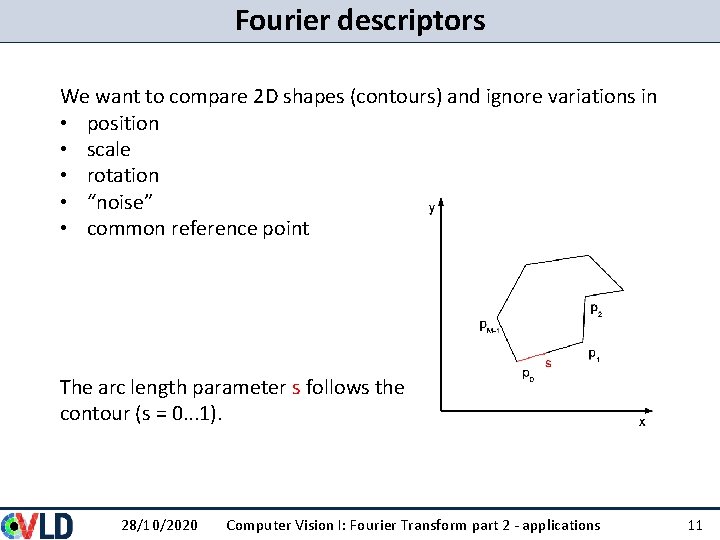
Fourier descriptors We want to compare 2 D shapes (contours) and ignore variations in • position • scale • rotation • “noise” • common reference point The arc length parameter s follows the contour (s = 0. . . 1). 28/10/2020 Computer Vision I: Fourier Transform part 2 - applications 11

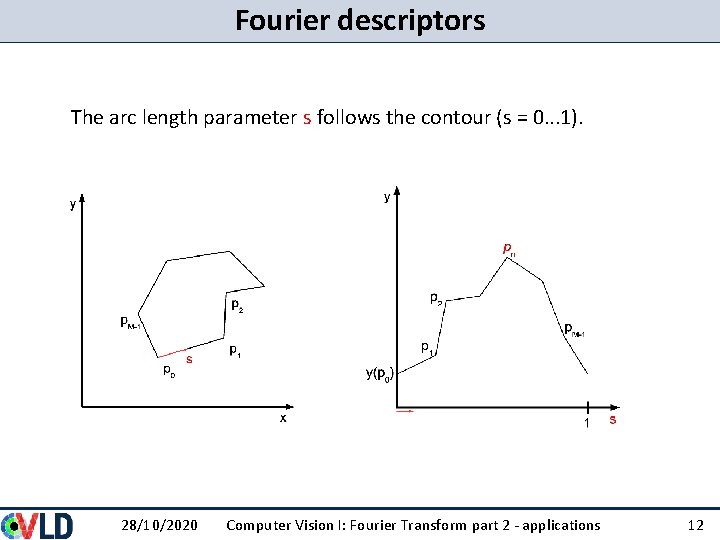
Fourier descriptors The arc length parameter s follows the contour (s = 0. . . 1). 28/10/2020 Computer Vision I: Fourier Transform part 2 - applications 12

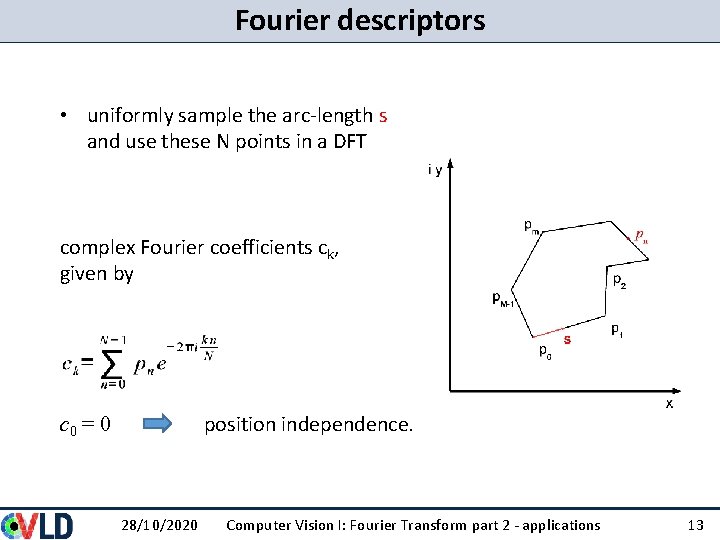
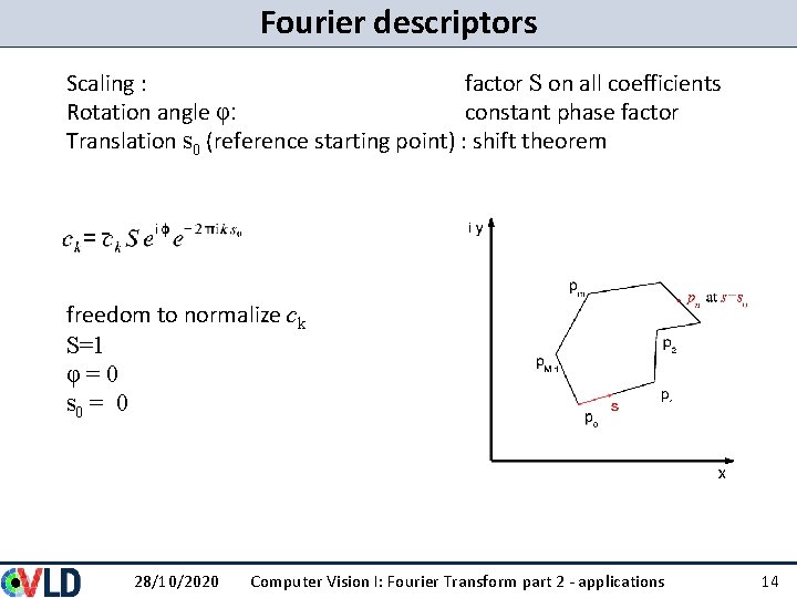
Fourier descriptors • uniformly sample the arc-length s and use these N points in a DFT complex Fourier coefficients ck, given by position independence. c 0 = 0 28/10/2020 Computer Vision I: Fourier Transform part 2 - applications 13

Fourier descriptors Scaling : factor S on all coefficients Rotation angle φ: constant phase factor Translation s 0 (reference starting point) : shift theorem freedom to normalize ck S=1 φ=0 s 0 = 0 28/10/2020 Computer Vision I: Fourier Transform part 2 - applications 14

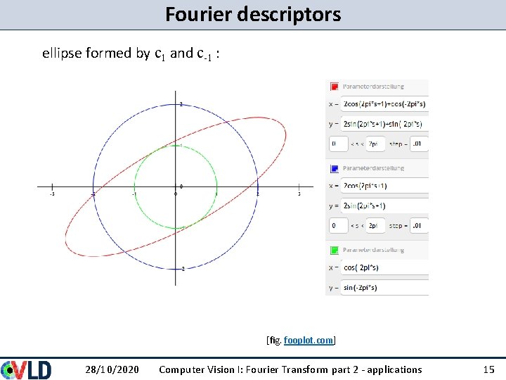
Fourier descriptors ellipse formed by c 1 and c-1 : [fig. fooplot. com] 28/10/2020 Computer Vision I: Fourier Transform part 2 - applications 15

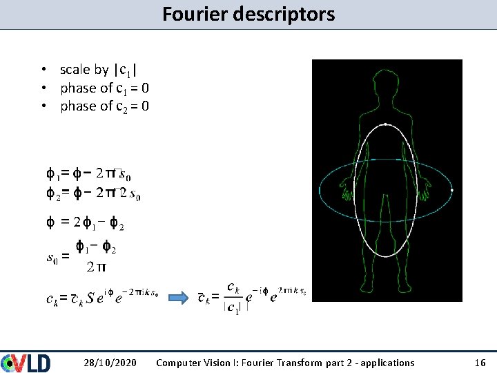
Fourier descriptors • scale by |c 1| • phase of c 1 = 0 • phase of c 2 = 0 28/10/2020 Computer Vision I: Fourier Transform part 2 - applications 16

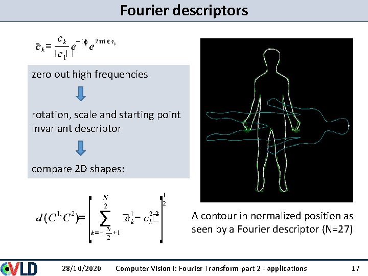
Fourier descriptors zero out high frequencies rotation, scale and starting point invariant descriptor compare 2 D shapes: A contour in normalized position as seen by a Fourier descriptor (N=27) 28/10/2020 Computer Vision I: Fourier Transform part 2 - applications 17

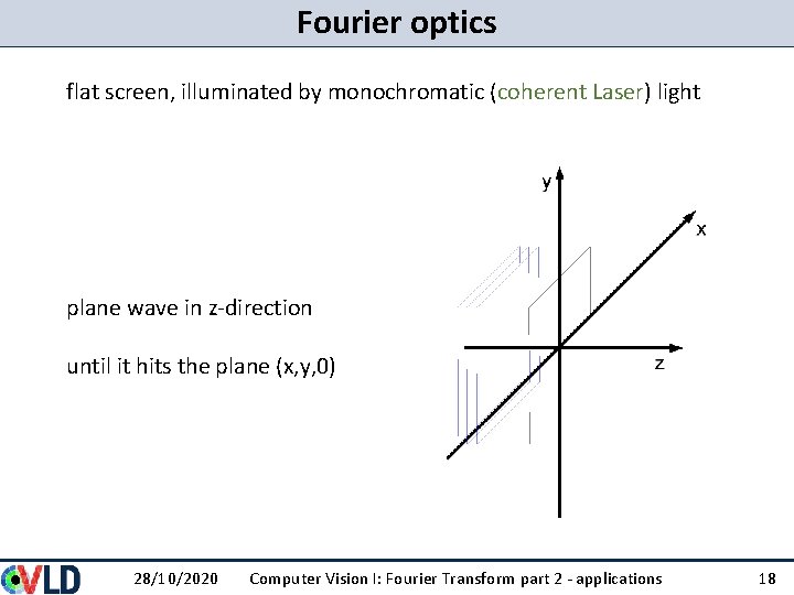
Fourier optics flat screen, illuminated by monochromatic (coherent Laser) light plane wave in z-direction until it hits the plane (x, y, 0) 28/10/2020 Computer Vision I: Fourier Transform part 2 - applications 18

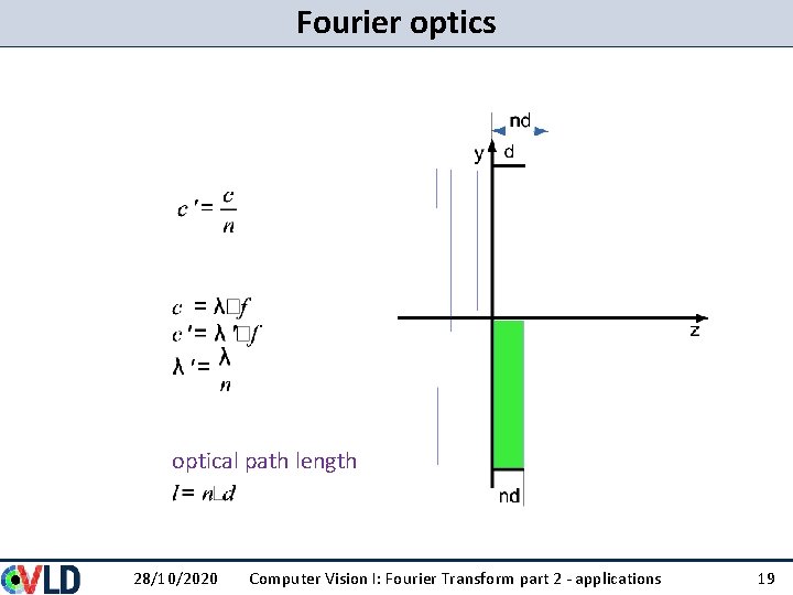
Fourier optics optical path length 28/10/2020 Computer Vision I: Fourier Transform part 2 - applications 19

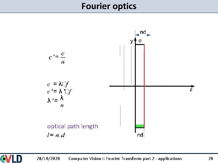
Fourier optics optical path length 28/10/2020 Computer Vision I: Fourier Transform part 2 - applications 20

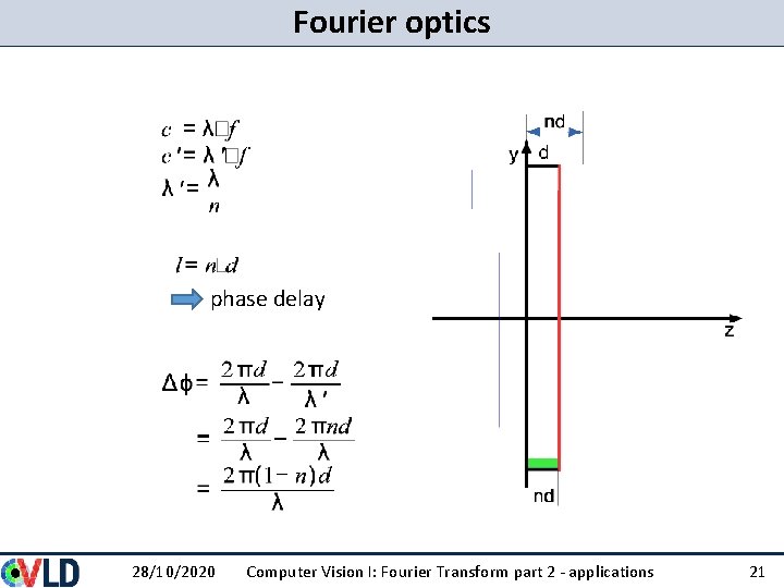
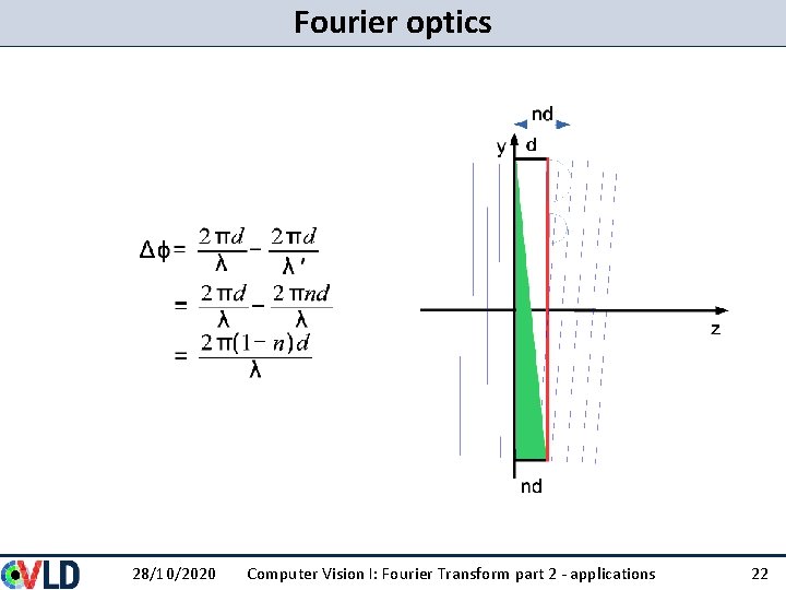
Fourier optics phase delay 28/10/2020 Computer Vision I: Fourier Transform part 2 - applications 21

Fourier optics 28/10/2020 Computer Vision I: Fourier Transform part 2 - applications 22

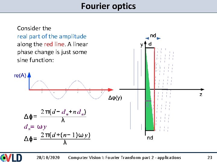
Fourier optics Consider the real part of the amplitude along the red line. A linear phase change is just some sine function: 28/10/2020 Computer Vision I: Fourier Transform part 2 - applications 23

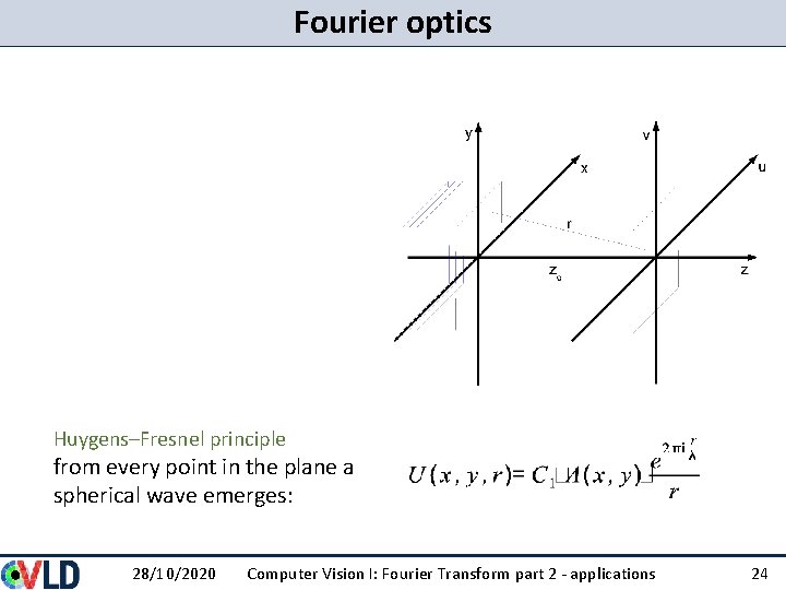
Fourier optics Huygens–Fresnel principle from every point in the plane a spherical wave emerges: 28/10/2020 Computer Vision I: Fourier Transform part 2 - applications 24

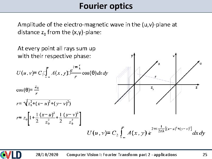
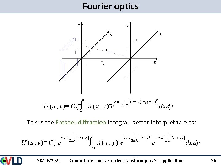
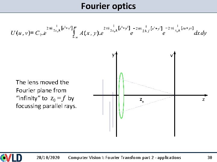
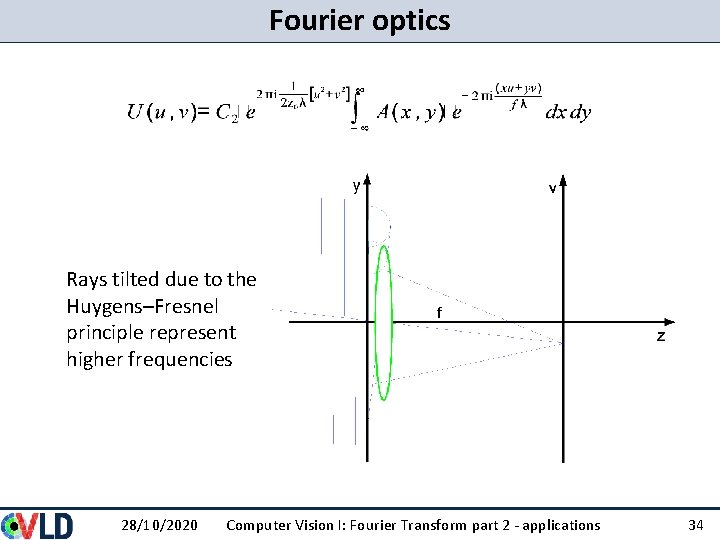
Fourier optics Amplitude of the electro-magnetic wave in the (u, v)-plane at distance z 0 from the (x, y)-plane: At every point all rays sum up with their respective phase: 28/10/2020 Computer Vision I: Fourier Transform part 2 - applications 25

Fourier optics This is the Fresnel-diffraction integral, better interpretable as: 28/10/2020 Computer Vision I: Fourier Transform part 2 - applications 26

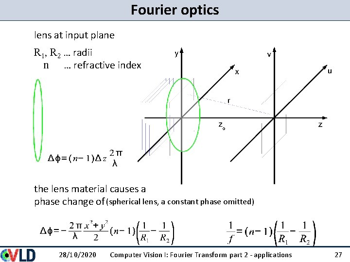
Fourier optics lens at input plane R 1, R 2 … radii n … refractive index the lens material causes a phase change of (spherical lens, a constant phase omitted) 28/10/2020 Computer Vision I: Fourier Transform part 2 - applications 27

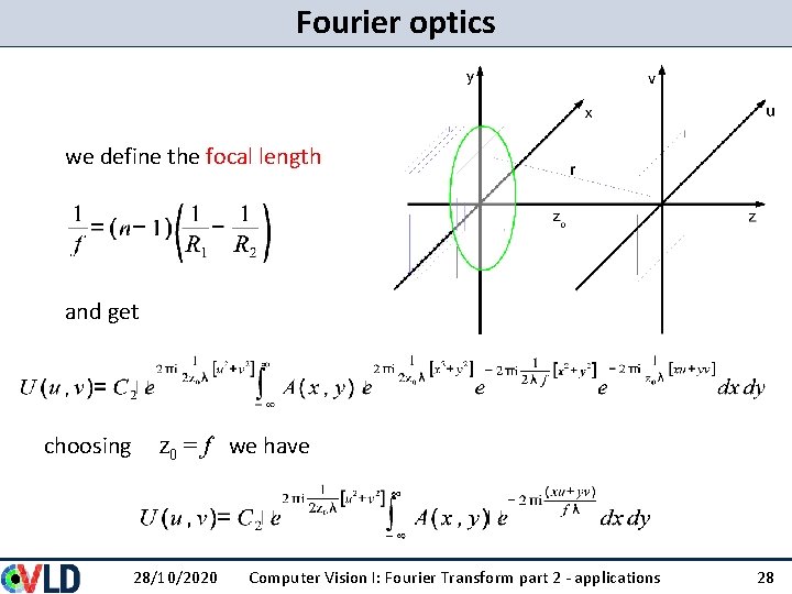
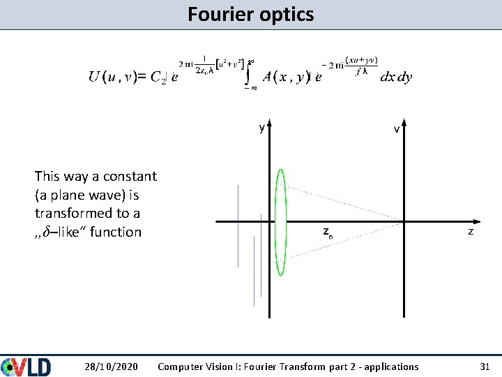
Fourier optics we define the focal length and get choosing z 0 = f we have 28/10/2020 Computer Vision I: Fourier Transform part 2 - applications 28

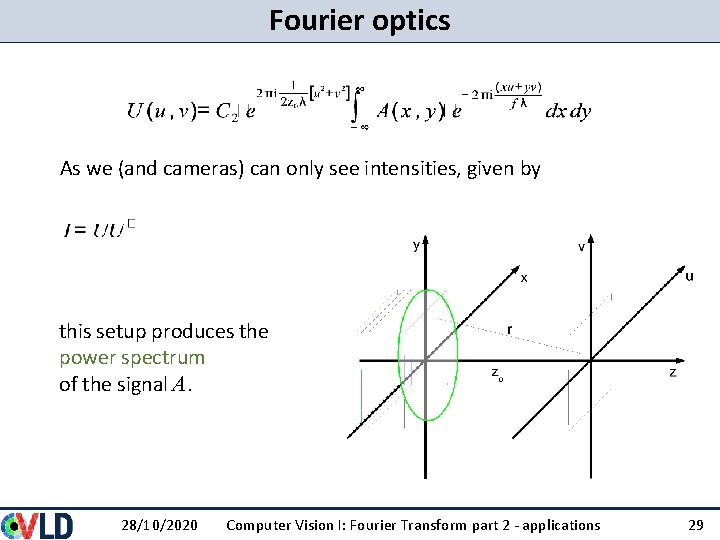
Fourier optics As we (and cameras) can only see intensities, given by this setup produces the power spectrum of the signal A. 28/10/2020 Computer Vision I: Fourier Transform part 2 - applications 29

Fourier optics The lens moved the Fourier plane from “infinity” to z 0 = f by focussing parallel rays. 28/10/2020 Computer Vision I: Fourier Transform part 2 - applications 30

Fourier optics This way a constant (a plane wave) is transformed to a „δ–like“ function 28/10/2020 Computer Vision I: Fourier Transform part 2 - applications 31

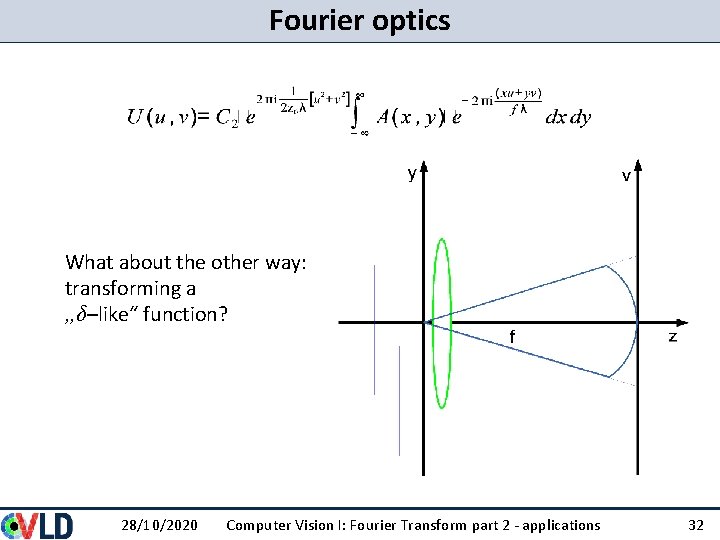
Fourier optics What about the other way: transforming a „δ–like“ function? 28/10/2020 Computer Vision I: Fourier Transform part 2 - applications 32

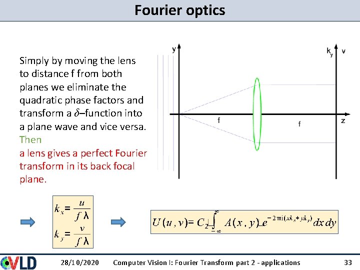
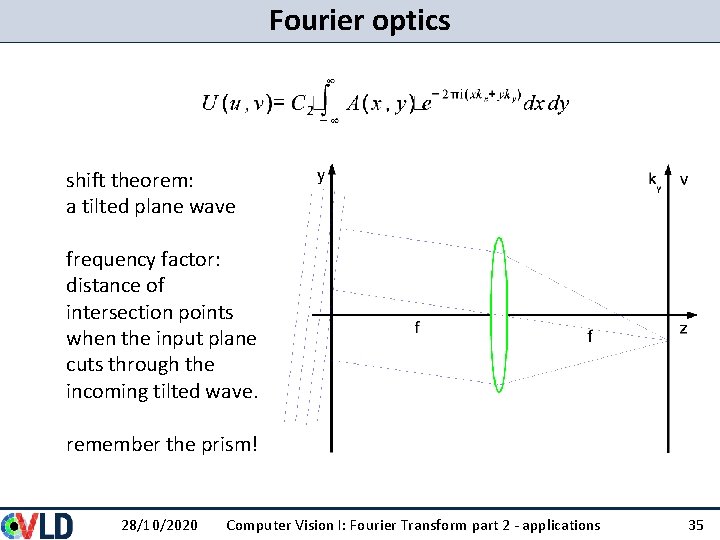
Fourier optics Simply by moving the lens to distance f from both planes we eliminate the quadratic phase factors and transform a δ–function into a plane wave and vice versa. Then a lens gives a perfect Fourier transform in its back focal plane. 28/10/2020 Computer Vision I: Fourier Transform part 2 - applications 33

Fourier optics Rays tilted due to the Huygens–Fresnel principle represent higher frequencies 28/10/2020 Computer Vision I: Fourier Transform part 2 - applications 34

Fourier optics shift theorem: a tilted plane wave frequency factor: distance of intersection points when the input plane cuts through the incoming tilted wave. remember the prism! 28/10/2020 Computer Vision I: Fourier Transform part 2 - applications 35

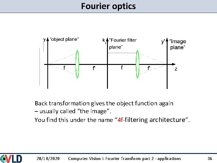
Fourier optics Back transformation gives the object function again – usually called “the image”. You find this under the name “ 4 f-filtering architecture”. 28/10/2020 Computer Vision I: Fourier Transform part 2 - applications 36

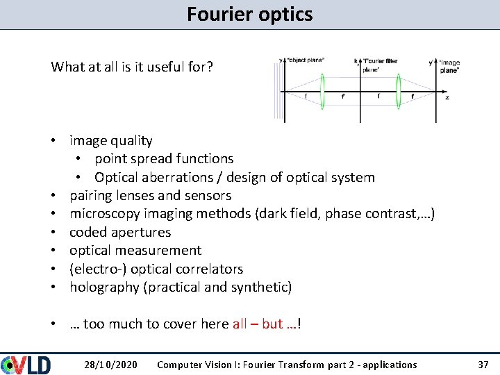
Fourier optics What at all is it useful for? • image quality • point spread functions • Optical aberrations / design of optical system • pairing lenses and sensors • microscopy imaging methods (dark field, phase contrast, …) • coded apertures • optical measurement • (electro-) optical correlators • holography (practical and synthetic) • … too much to cover here all – but …! 28/10/2020 Computer Vision I: Fourier Transform part 2 - applications 37

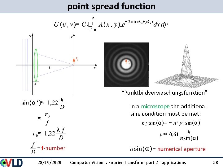
point spread function “Punktbildverwaschungsfunktion” in a microscope the additional sine condition must be met: = f-number 28/10/2020 = numerical aperture Computer Vision I: Fourier Transform part 2 - applications 38

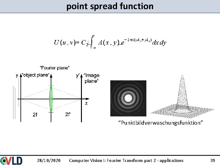
point spread function “Punktbildverwaschungsfunktion” 28/10/2020 Computer Vision I: Fourier Transform part 2 - applications 39

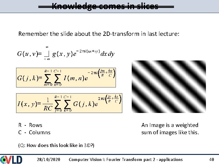
Knowledge comes in slices Remember the slide about the 2 D-transform in last lecture: R - Rows C - Columns An Image is a weighted sum of images like this. (Q: How does this look like in 3 D? ) 28/10/2020 Computer Vision I: Fourier Transform part 2 - applications 40

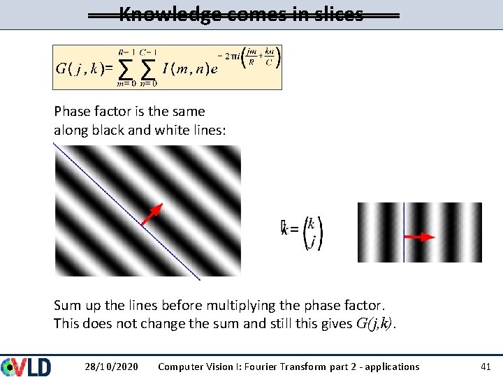
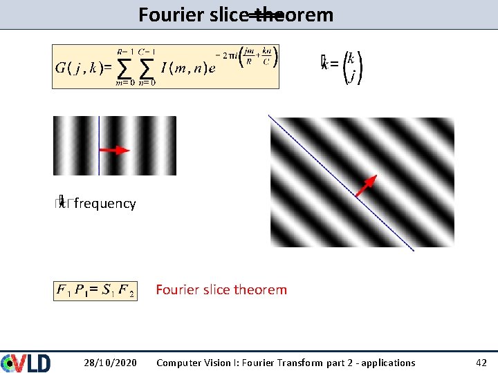
Knowledge comes in slices Phase factor is the same along black and white lines: Sum up the lines before multiplying the phase factor. This does not change the sum and still this gives G(j, k). 28/10/2020 Computer Vision I: Fourier Transform part 2 - applications 41

Fourier slice theorem frequency Fourier slice theorem 28/10/2020 Computer Vision I: Fourier Transform part 2 - applications 42

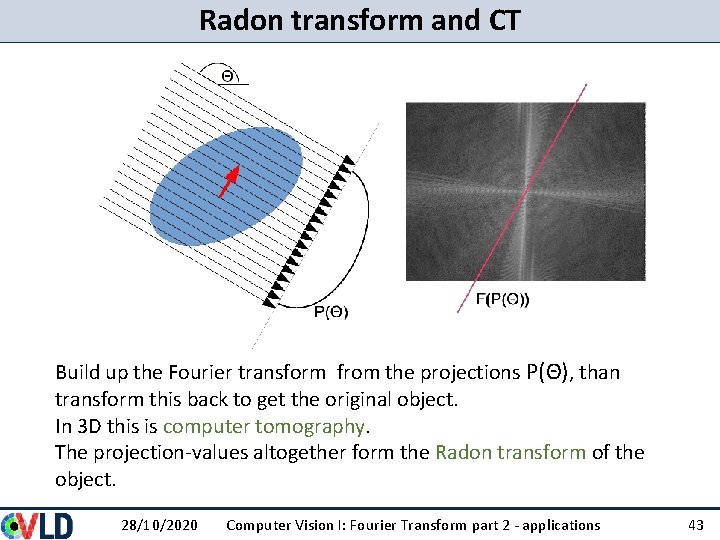
Radon transform and CT Build up the Fourier transform from the projections P(Θ), than transform this back to get the original object. In 3 D this is computer tomography. The projection-values altogether form the Radon transform of the object. 28/10/2020 Computer Vision I: Fourier Transform part 2 - applications 43