Computer vision models learning and inference Chapter 10
- Slides: 59

Computer vision: models, learning and inference Chapter 10 Graphical Models

Independence • Two variables x 1 and x 2 are independent if their joint probability distribution factorizes as Pr(x 1, x 2)=Pr(x 1) Pr(x 2) Computer vision: models, learning and inference. © 2011 Simon J. D. Prince 2

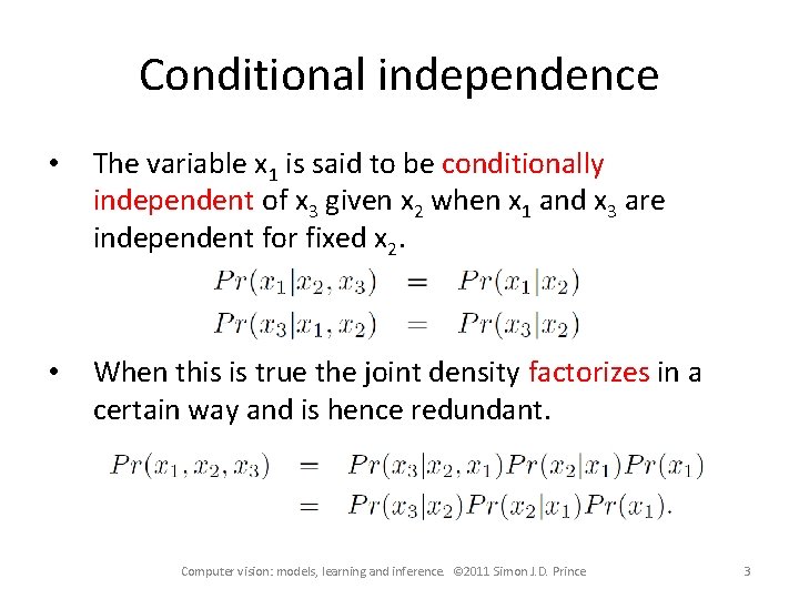
Conditional independence • The variable x 1 is said to be conditionally independent of x 3 given x 2 when x 1 and x 3 are independent for fixed x 2. • When this is true the joint density factorizes in a certain way and is hence redundant. Computer vision: models, learning and inference. © 2011 Simon J. D. Prince 3

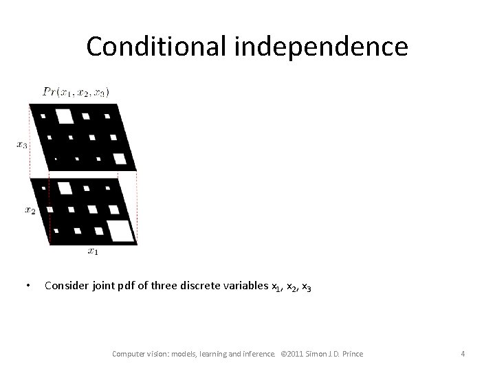
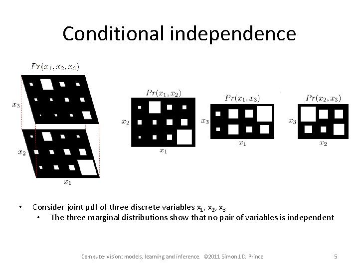
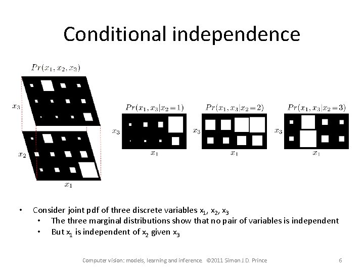
Conditional independence • Consider joint pdf of three discrete variables x 1, x 2, x 3 Computer vision: models, learning and inference. © 2011 Simon J. D. Prince 4

Conditional independence • Consider joint pdf of three discrete variables x 1, x 2, x 3 • The three marginal distributions show that no pair of variables is independent Computer vision: models, learning and inference. © 2011 Simon J. D. Prince 5

Conditional independence • Consider joint pdf of three discrete variables x 1, x 2, x 3 • The three marginal distributions show that no pair of variables is independent • But x 1 is independent of x 2 given x 3 Computer vision: models, learning and inference. © 2011 Simon J. D. Prince 6

Graphical models • A graphical model is a graph based representation that makes both factorization and conditional independence relations easy to establish • Two important types: – Directed graphical model or Bayesian network – Undirected graphical model or Markov network Computer vision: models, learning and inference. © 2011 Simon J. D. Prince 7

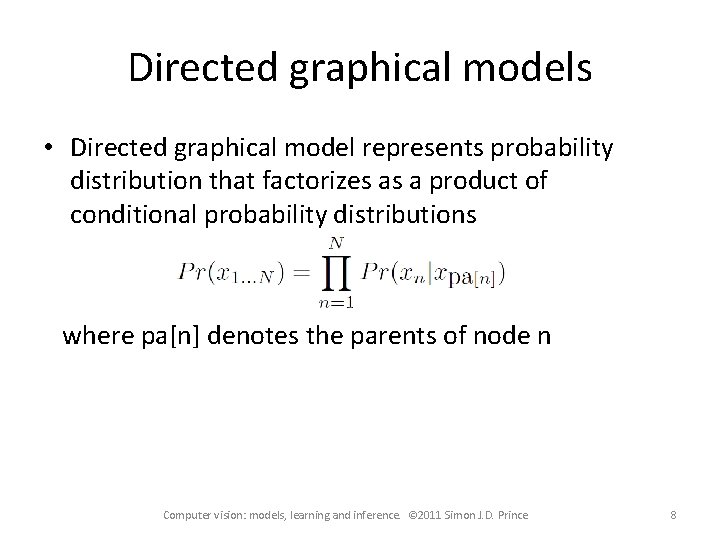
Directed graphical models • Directed graphical model represents probability distribution that factorizes as a product of conditional probability distributions where pa[n] denotes the parents of node n Computer vision: models, learning and inference. © 2011 Simon J. D. Prince 8

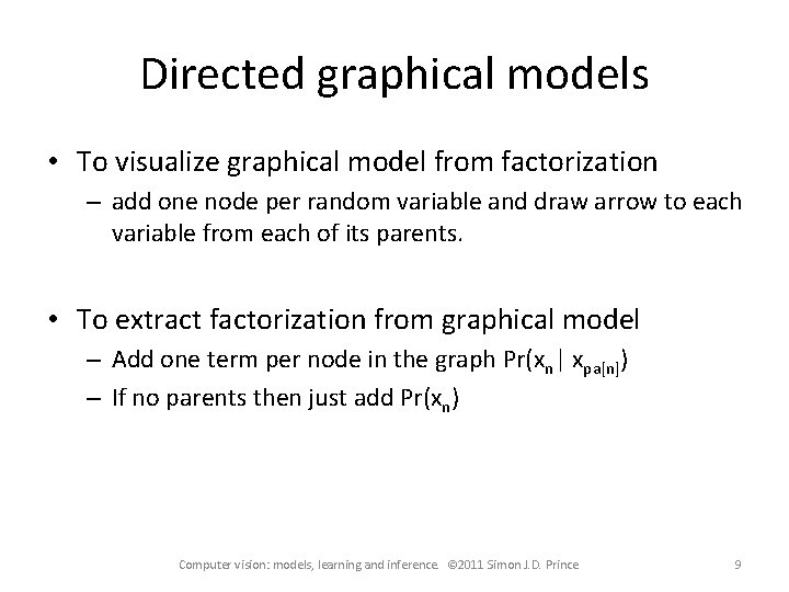
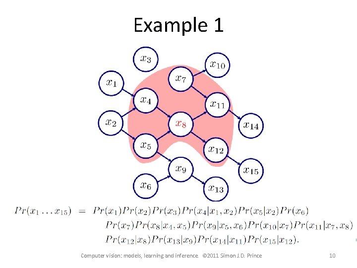
Directed graphical models • To visualize graphical model from factorization – add one node per random variable and draw arrow to each variable from each of its parents. • To extract factorization from graphical model – Add one term per node in the graph Pr(xn| xpa[n]) – If no parents then just add Pr(xn) Computer vision: models, learning and inference. © 2011 Simon J. D. Prince 9

Example 1 Computer vision: models, learning and inference. © 2011 Simon J. D. Prince 10

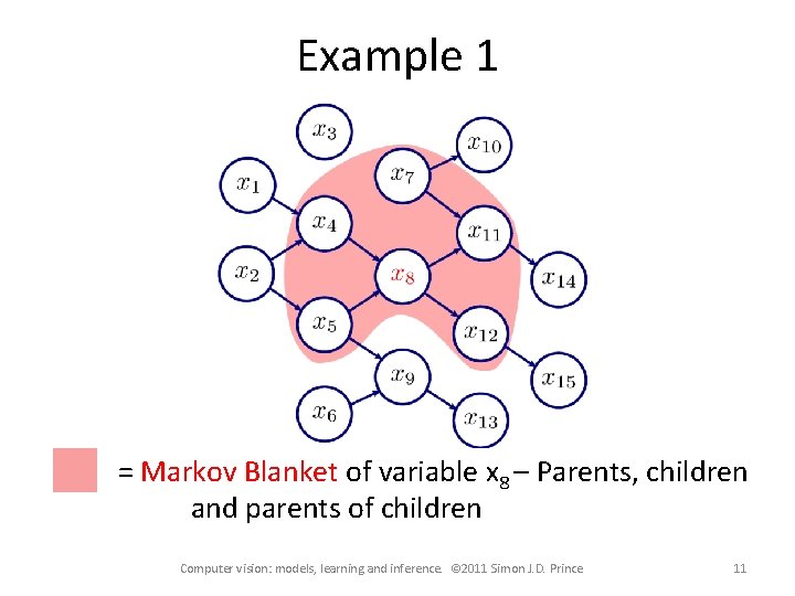
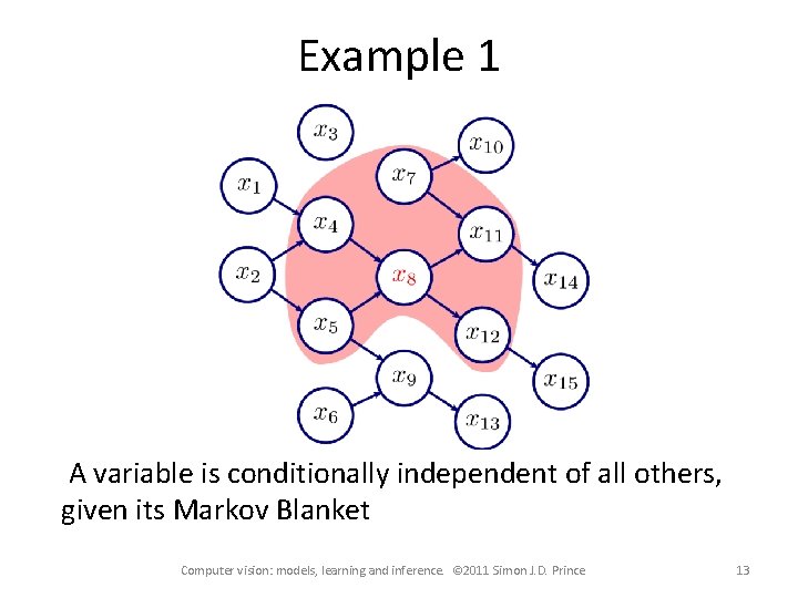
Example 1 = Markov Blanket of variable x 8 – Parents, children and parents of children Computer vision: models, learning and inference. © 2011 Simon J. D. Prince 11

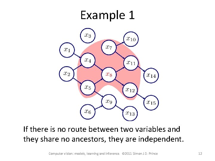
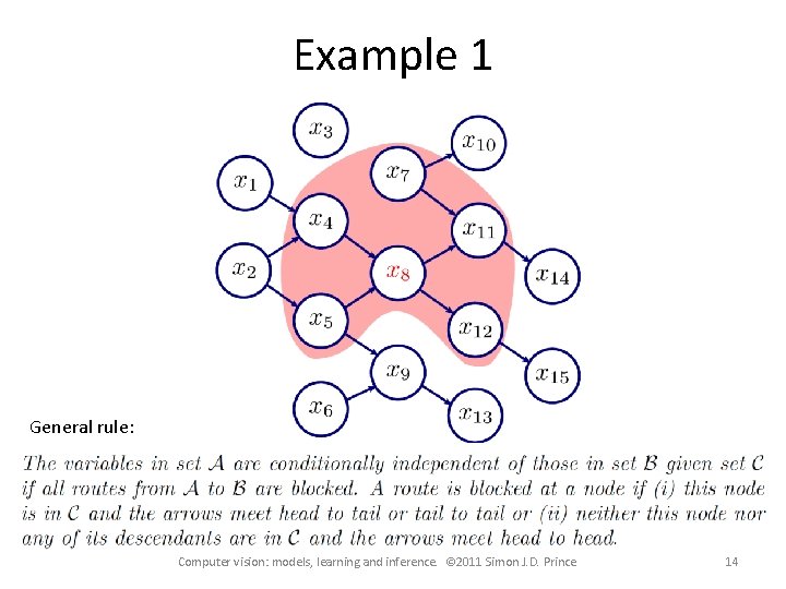
Example 1 If there is no route between two variables and they share no ancestors, they are independent. Computer vision: models, learning and inference. © 2011 Simon J. D. Prince 12

Example 1 A variable is conditionally independent of all others, given its Markov Blanket Computer vision: models, learning and inference. © 2011 Simon J. D. Prince 13

Example 1 General rule: Computer vision: models, learning and inference. © 2011 Simon J. D. Prince 14

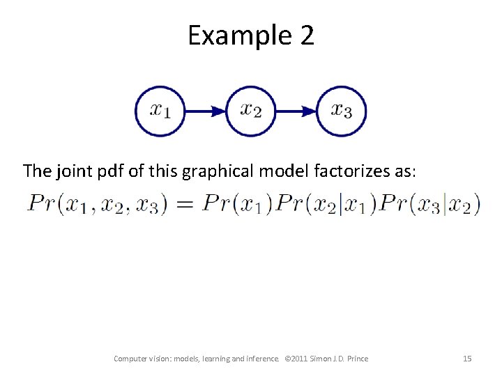
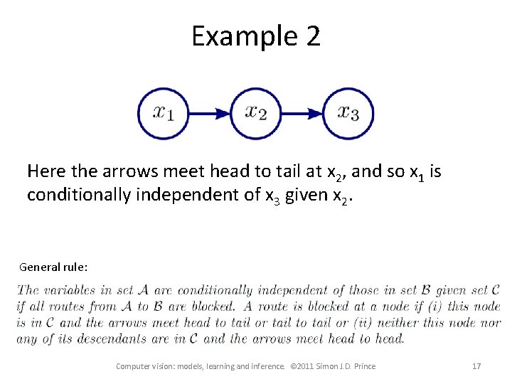
Example 2 The joint pdf of this graphical model factorizes as: Computer vision: models, learning and inference. © 2011 Simon J. D. Prince 15

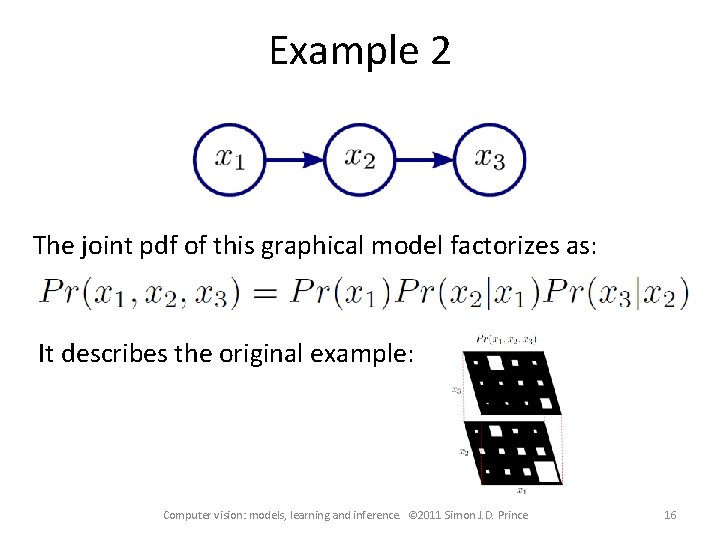
Example 2 The joint pdf of this graphical model factorizes as: It describes the original example: Computer vision: models, learning and inference. © 2011 Simon J. D. Prince 16

Example 2 Here the arrows meet head to tail at x 2, and so x 1 is conditionally independent of x 3 given x 2. General rule: Computer vision: models, learning and inference. © 2011 Simon J. D. Prince 17

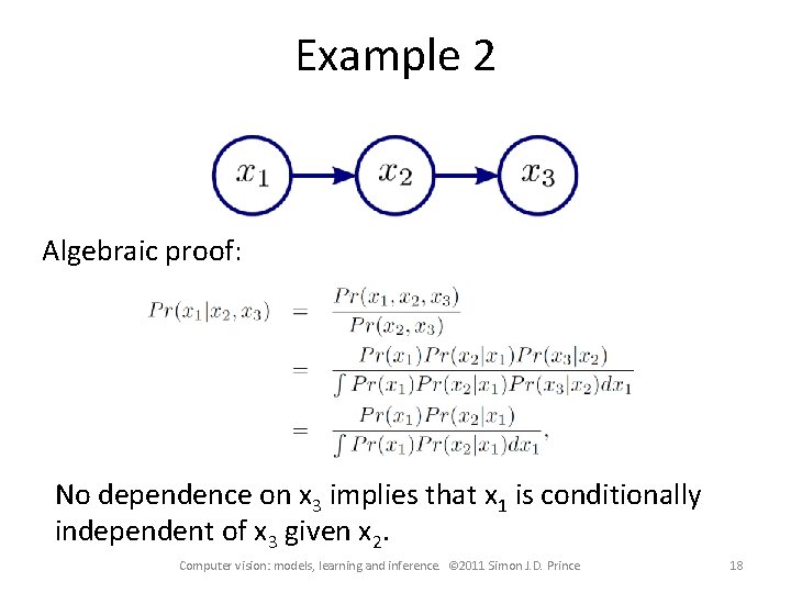
Example 2 Algebraic proof: No dependence on x 3 implies that x 1 is conditionally independent of x 3 given x 2. Computer vision: models, learning and inference. © 2011 Simon J. D. Prince 18

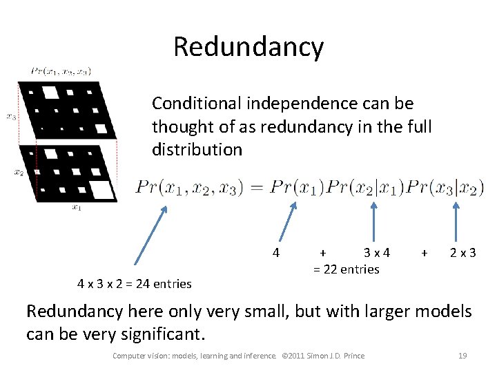
Redundancy Conditional independence can be thought of as redundancy in the full distribution 4 4 x 3 x 2 = 24 entries + 3 x 4 = 22 entries + 2 x 3 Redundancy here only very small, but with larger models can be very significant. Computer vision: models, learning and inference. © 2011 Simon J. D. Prince 19

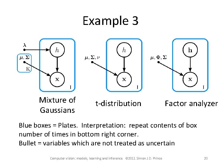
Example 3 Mixture of Gaussians t-distribution Factor analyzer Blue boxes = Plates. Interpretation: repeat contents of box number of times in bottom right corner. Bullet = variables which are not treated as uncertain Computer vision: models, learning and inference. © 2011 Simon J. D. Prince 20

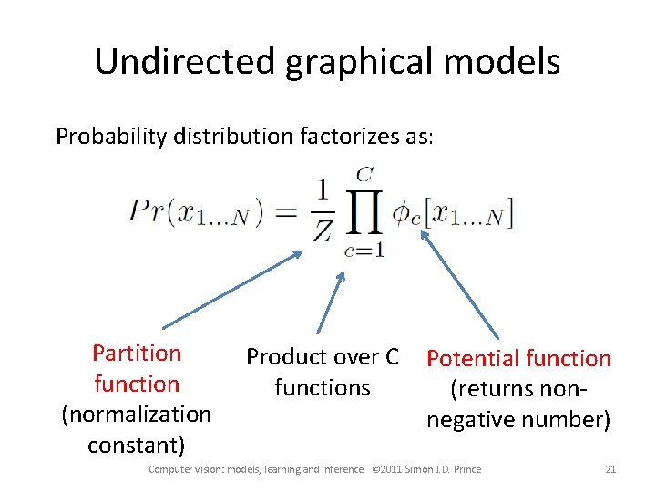
Undirected graphical models Probability distribution factorizes as: Partition function (normalization constant) Product over C functions Potential function (returns nonnegative number) Computer vision: models, learning and inference. © 2011 Simon J. D. Prince 21

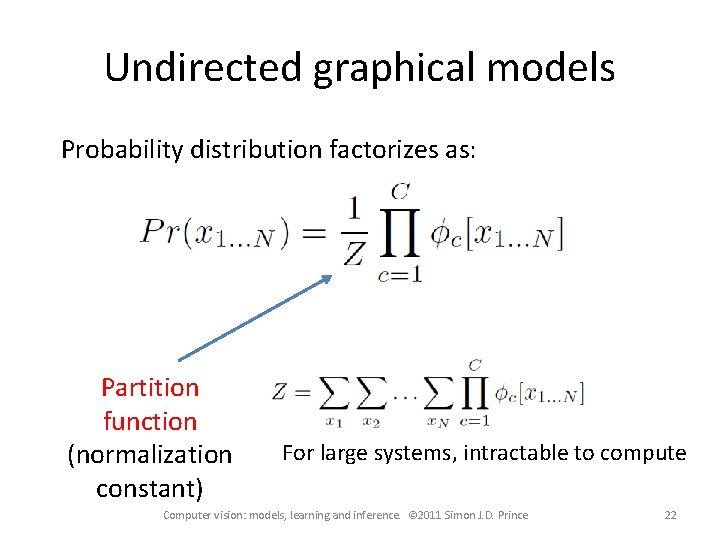
Undirected graphical models Probability distribution factorizes as: Partition function (normalization constant) For large systems, intractable to compute Computer vision: models, learning and inference. © 2011 Simon J. D. Prince 22

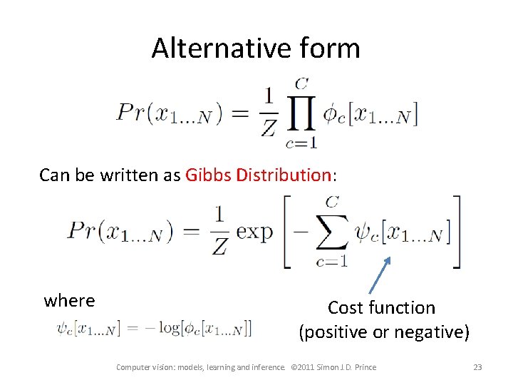
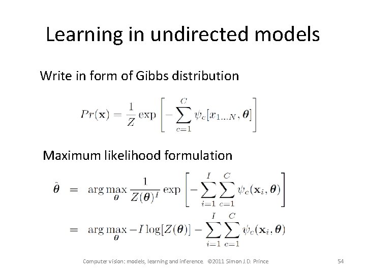
Alternative form Can be written as Gibbs Distribution: where Cost function (positive or negative) Computer vision: models, learning and inference. © 2011 Simon J. D. Prince 23

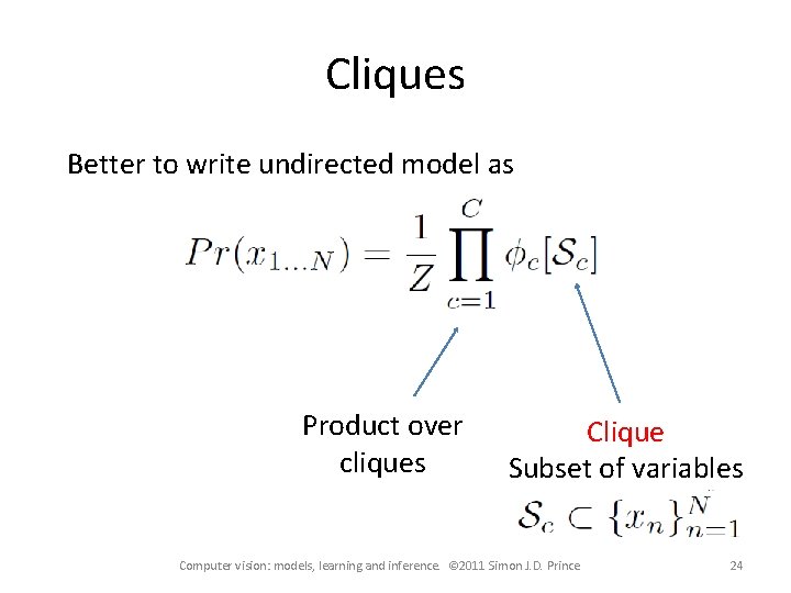
Cliques Better to write undirected model as Product over cliques Clique Subset of variables Computer vision: models, learning and inference. © 2011 Simon J. D. Prince 24

Undirected graphical models • To visualize graphical model from factorization – Sketch one node per random variable – For every clique, sketch connection from every node to every other • To extract factorization from graphical model – Add one term to factorization per maximal clique (fully connected subset of nodes where it is not possible to add another node and remain fully connected) Computer vision: models, learning and inference. © 2011 Simon J. D. Prince 25

Conditional independence • Much simpler than for directed models: One set of nodes is conditionally independent of another given a third if the third set separates them (i. e. Blocks any path from the first node to the second) Computer vision: models, learning and inference. © 2011 Simon J. D. Prince 26

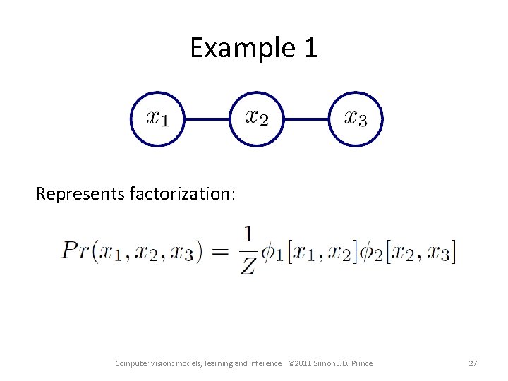
Example 1 Represents factorization: Computer vision: models, learning and inference. © 2011 Simon J. D. Prince 27

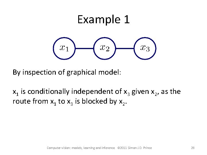
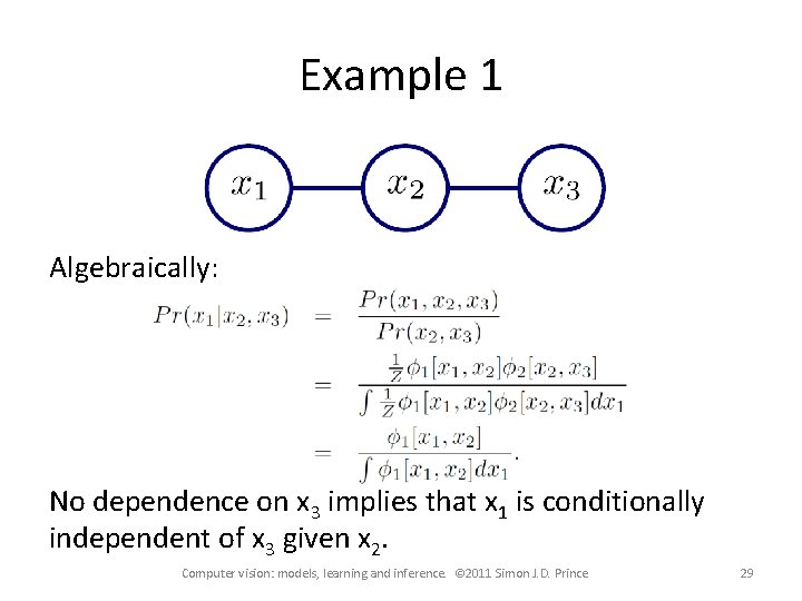
Example 1 By inspection of graphical model: x 1 is conditionally independent of x 3 given x 2, as the route from x 1 to x 3 is blocked by x 2. Computer vision: models, learning and inference. © 2011 Simon J. D. Prince 28

Example 1 Algebraically: No dependence on x 3 implies that x 1 is conditionally independent of x 3 given x 2. Computer vision: models, learning and inference. © 2011 Simon J. D. Prince 29

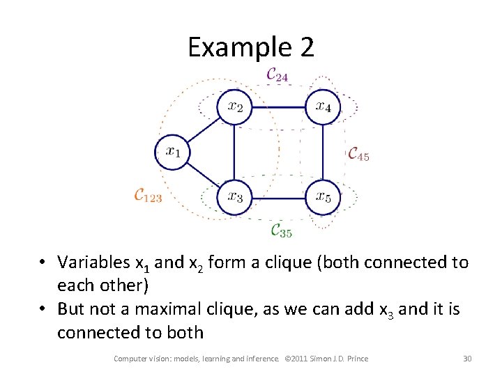
Example 2 • Variables x 1 and x 2 form a clique (both connected to each other) • But not a maximal clique, as we can add x 3 and it is connected to both Computer vision: models, learning and inference. © 2011 Simon J. D. Prince 30

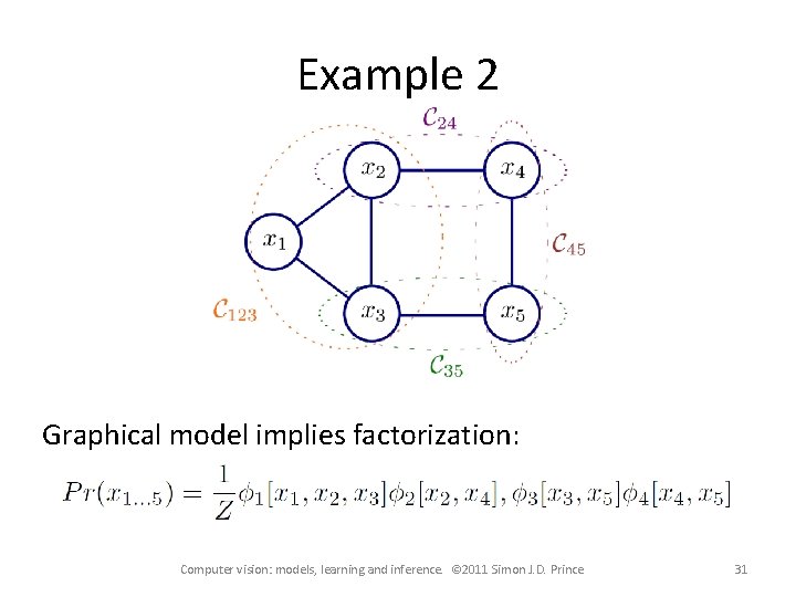
Example 2 Graphical model implies factorization: Computer vision: models, learning and inference. © 2011 Simon J. D. Prince 31

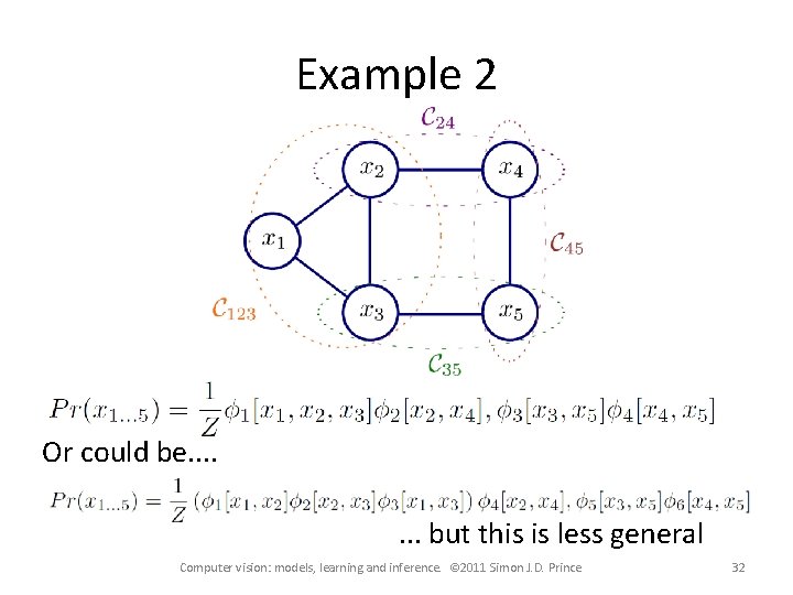
Example 2 Or could be. . . . but this is less general Computer vision: models, learning and inference. © 2011 Simon J. D. Prince 32

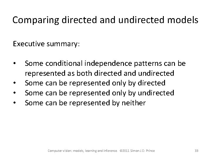
Comparing directed and undirected models Executive summary: • • Some conditional independence patterns can be represented as both directed and undirected Some can be represented only by undirected Some can be represented by neither Computer vision: models, learning and inference. © 2011 Simon J. D. Prince 33

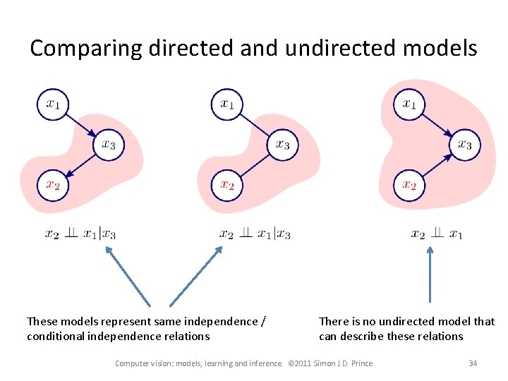
Comparing directed and undirected models These models represent same independence / conditional independence relations There is no undirected model that can describe these relations Computer vision: models, learning and inference. © 2011 Simon J. D. Prince 34

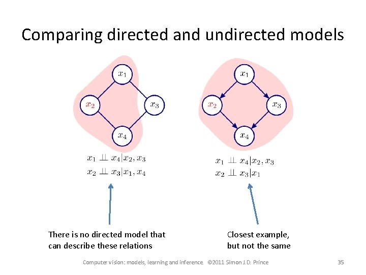
Comparing directed and undirected models There is no directed model that can describe these relations Closest example, but not the same Computer vision: models, learning and inference. © 2011 Simon J. D. Prince 35

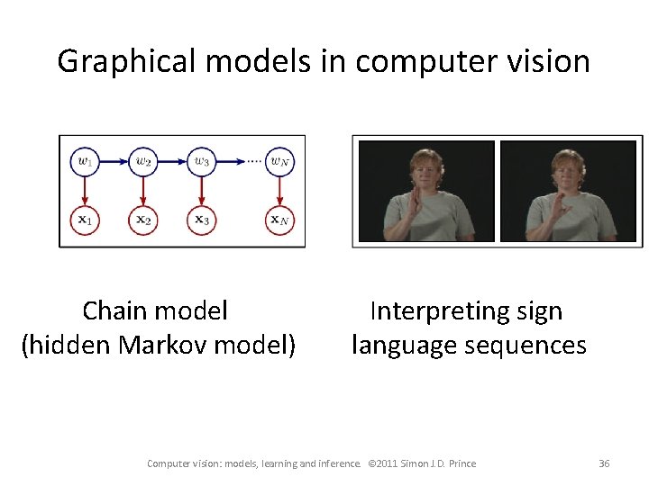
Graphical models in computer vision Chain model (hidden Markov model) Interpreting sign language sequences Computer vision: models, learning and inference. © 2011 Simon J. D. Prince 36

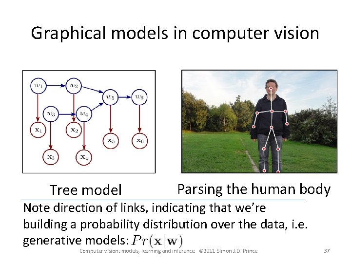
Graphical models in computer vision Tree model Parsing the human body Note direction of links, indicating that we’re building a probability distribution over the data, i. e. generative models: Computer vision: models, learning and inference. © 2011 Simon J. D. Prince 37

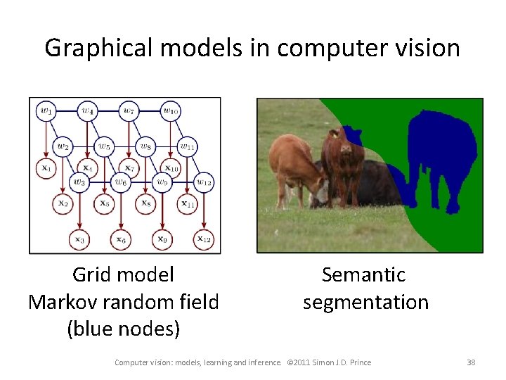
Graphical models in computer vision Grid model Markov random field (blue nodes) Semantic segmentation Computer vision: models, learning and inference. © 2011 Simon J. D. Prince 38

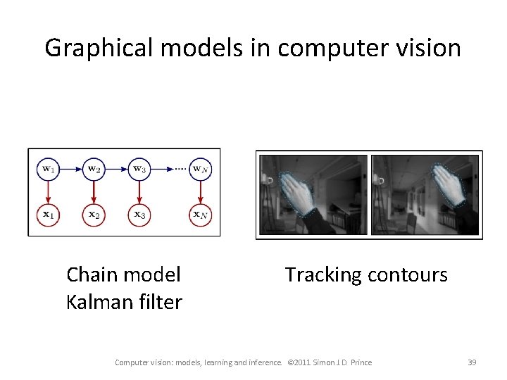
Graphical models in computer vision Chain model Kalman filter Tracking contours Computer vision: models, learning and inference. © 2011 Simon J. D. Prince 39

Inference in models with many unknowns • Ideally we would compute full posterior distribution Pr(w 1. . . N|x 1. . . N). • But for most models this is a very large discrete distribution – intractable to compute • Other solutions: – Find MAP solution – Find marginal posterior distributions – Maximum marginals – Sampling posterior Computer vision: models, learning and inference. © 2011 Simon J. D. Prince 40

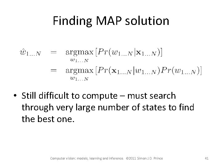
Finding MAP solution • Still difficult to compute – must search through very large number of states to find the best one. Computer vision: models, learning and inference. © 2011 Simon J. D. Prince 41

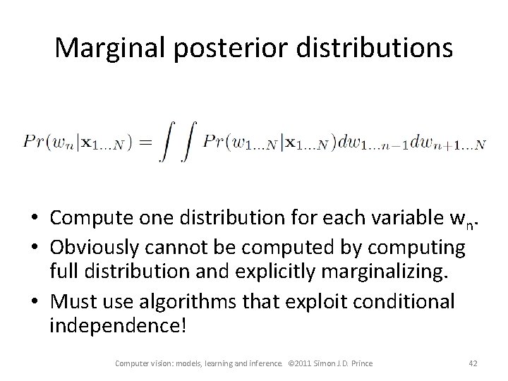
Marginal posterior distributions • Compute one distribution for each variable wn. • Obviously cannot be computed by computing full distribution and explicitly marginalizing. • Must use algorithms that exploit conditional independence! Computer vision: models, learning and inference. © 2011 Simon J. D. Prince 42

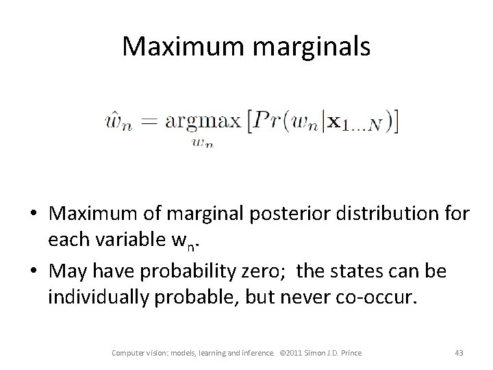
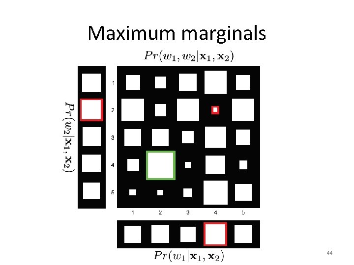
Maximum marginals • Maximum of marginal posterior distribution for each variable wn. • May have probability zero; the states can be individually probable, but never co-occur. Computer vision: models, learning and inference. © 2011 Simon J. D. Prince 43

Maximum marginals Computer vision: models, learning and inference. © 2011 Simon J. D. Prince 44

Sampling the posterior • Draw samples from posterior Pr(w 1. . . N|x 1. . . N). – use samples as representation of distribution – select sample with highest prob. as point sample – compute empirical max-marginals • Look at marginal statistics of samples Computer vision: models, learning and inference. © 2011 Simon J. D. Prince 45

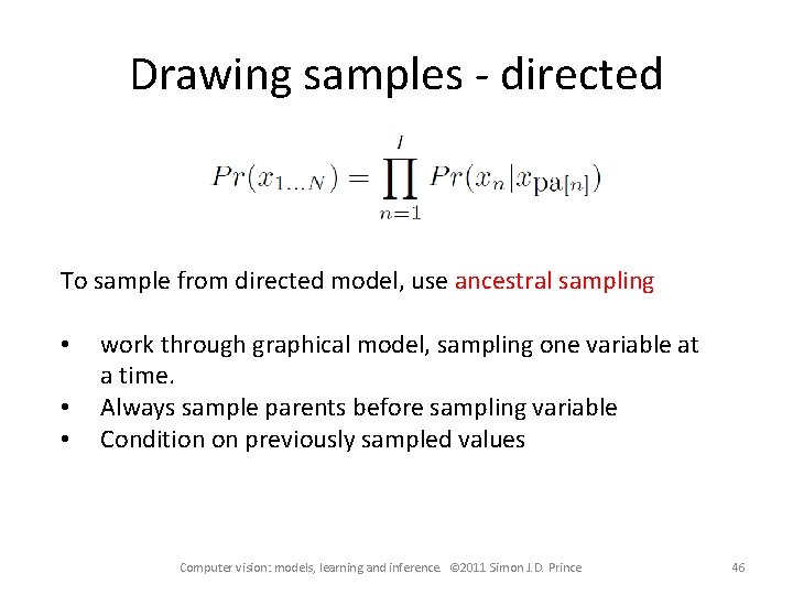
Drawing samples - directed To sample from directed model, use ancestral sampling • • • work through graphical model, sampling one variable at a time. Always sample parents before sampling variable Condition on previously sampled values Computer vision: models, learning and inference. © 2011 Simon J. D. Prince 46

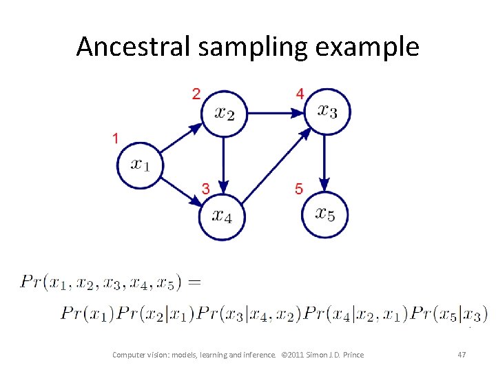
Ancestral sampling example Computer vision: models, learning and inference. © 2011 Simon J. D. Prince 47

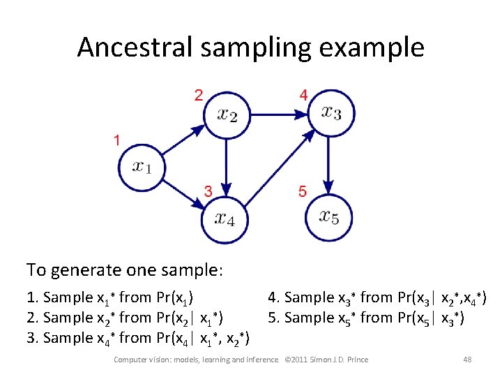
Ancestral sampling example To generate one sample: 1. Sample x 1* from Pr(x 1) 2. Sample x 2* from Pr(x 2| x 1*) 3. Sample x 4* from Pr(x 4| x 1*, x 2*) 4. Sample x 3* from Pr(x 3| x 2*, x 4*) 5. Sample x 5* from Pr(x 5| x 3*) Computer vision: models, learning and inference. © 2011 Simon J. D. Prince 48

Drawing samples - undirected • Can’t use ancestral sampling as no sense of parents / children and don’t have conditional probability distributions • Instead us Markov chain Monte Carlo method – Generate series of samples (chain) – Each depends on previous sample (Markov) – Generation stochastic (Monte Carlo) • Example MCMC method = Gibbs sampling Computer vision: models, learning and inference. © 2011 Simon J. D. Prince 49

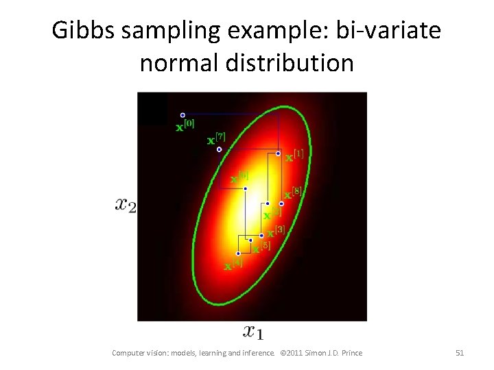
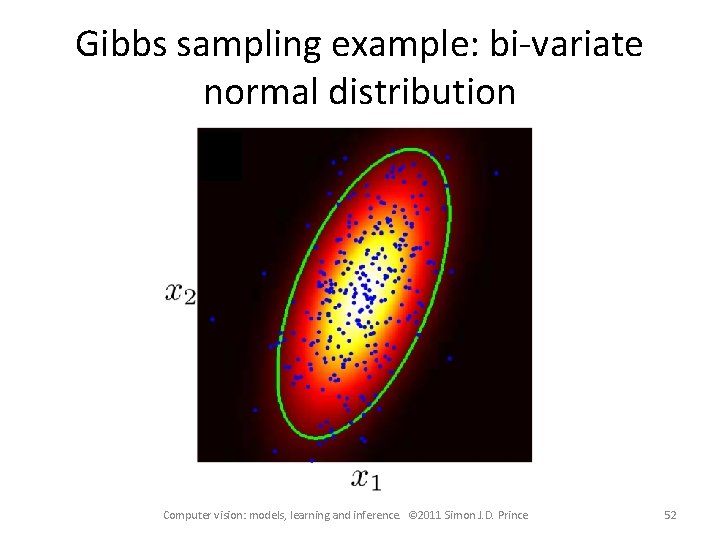
Gibbs sampling To generate new sample x in the chain – Sample each dimension in any order – To update nth dimension xn • • Fix other N-1 dimensions Draw from conditional distribution Pr(xn| x 1. . . Nn) Get samples by selecting from chain – Needs burn-in period – Choose samples spaced apart, so not correlated Computer vision: models, learning and inference. © 2011 Simon J. D. Prince 50

Gibbs sampling example: bi-variate normal distribution Computer vision: models, learning and inference. © 2011 Simon J. D. Prince 51

Gibbs sampling example: bi-variate normal distribution Computer vision: models, learning and inference. © 2011 Simon J. D. Prince 52

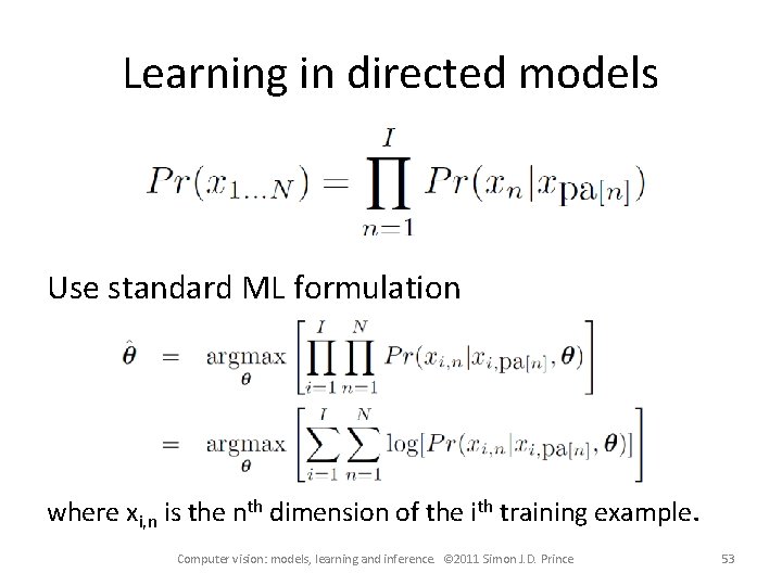
Learning in directed models Use standard ML formulation where xi, n is the nth dimension of the ith training example. Computer vision: models, learning and inference. © 2011 Simon J. D. Prince 53

Learning in undirected models Write in form of Gibbs distribution Maximum likelihood formulation Computer vision: models, learning and inference. © 2011 Simon J. D. Prince 54

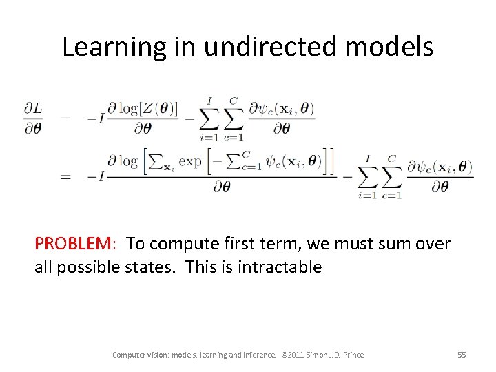
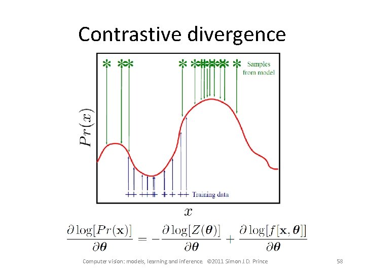
Learning in undirected models PROBLEM: To compute first term, we must sum over all possible states. This is intractable Computer vision: models, learning and inference. © 2011 Simon J. D. Prince 55

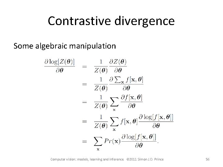
Contrastive divergence Some algebraic manipulation Computer vision: models, learning and inference. © 2011 Simon J. D. Prince 56

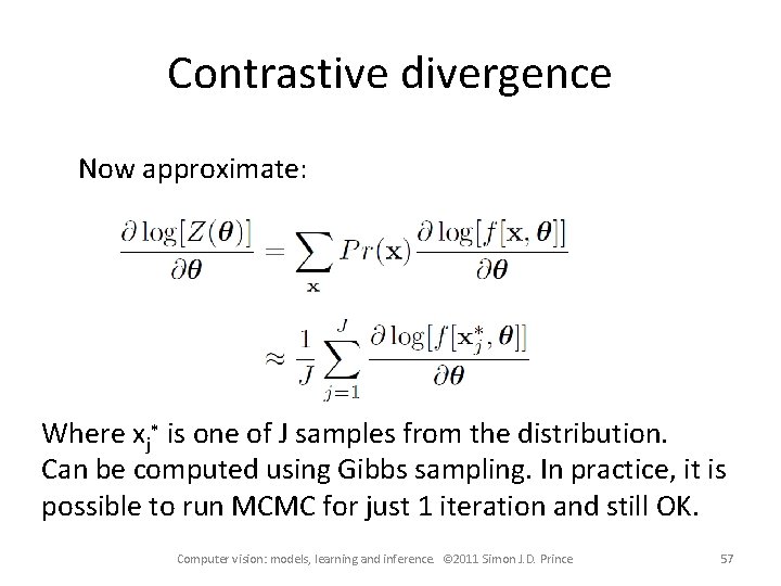
Contrastive divergence Now approximate: Where xj* is one of J samples from the distribution. Can be computed using Gibbs sampling. In practice, it is possible to run MCMC for just 1 iteration and still OK. Computer vision: models, learning and inference. © 2011 Simon J. D. Prince 57

Contrastive divergence Computer vision: models, learning and inference. © 2011 Simon J. D. Prince 58

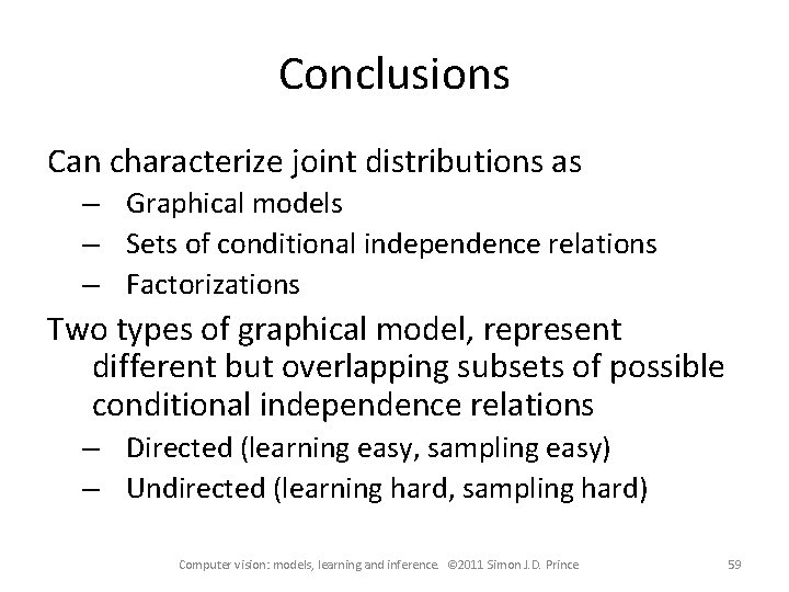
Conclusions Can characterize joint distributions as – Graphical models – Sets of conditional independence relations – Factorizations Two types of graphical model, represent different but overlapping subsets of possible conditional independence relations – Directed (learning easy, sampling easy) – Undirected (learning hard, sampling hard) Computer vision: models, learning and inference. © 2011 Simon J. D. Prince 59