Computer vision models learning and inference Chapter 12

Computer vision: models, learning and inference Chapter 12 Graphical Models Please send errata to s. prince@cs. ucl. ac. uk

Models for grids • • • Consider models where one unknown world state at each pixel in the image – takes the form of a grid. Loops in the graphical model so cannot use dynamic programming or belief propagation Define probability distributions that favour certain configurations of world states – – Called Markov random fields Inference using a set of techniques called graph cuts 2 Computer vision: models, learning and inference. © 2011 Simon J. D. Prince

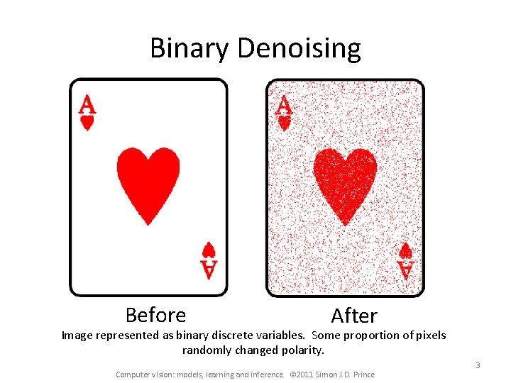
Binary Denoising Before After Image represented as binary discrete variables. Some proportion of pixels randomly changed polarity. Computer vision: models, learning and inference. © 2011 Simon J. D. Prince 3

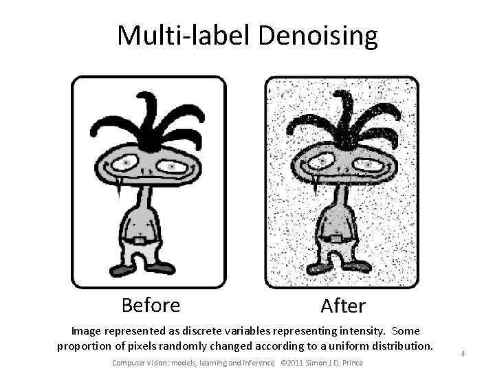
Multi-label Denoising Before After Image represented as discrete variables representing intensity. Some proportion of pixels randomly changed according to a uniform distribution. Computer vision: models, learning and inference. © 2011 Simon J. D. Prince 4

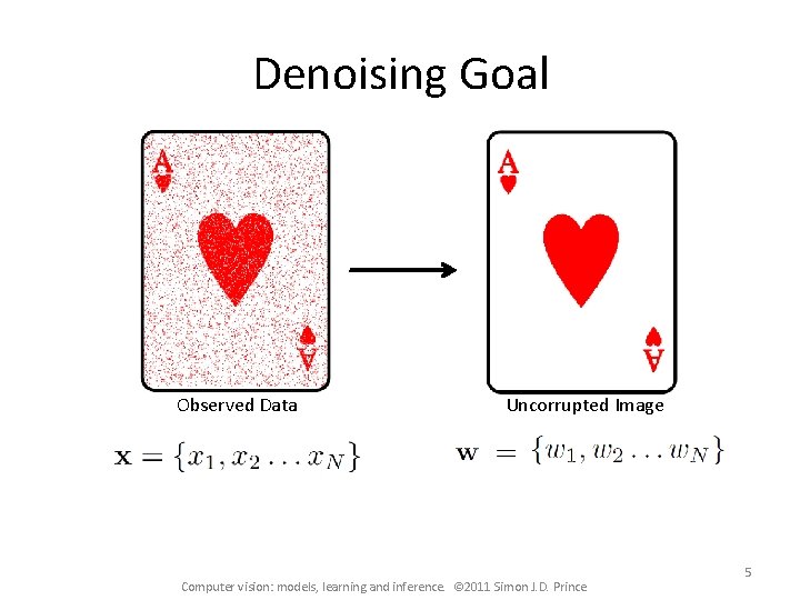
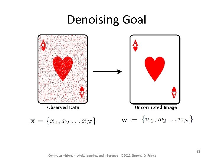
Denoising Goal Observed Data Uncorrupted Image Computer vision: models, learning and inference. © 2011 Simon J. D. Prince 5

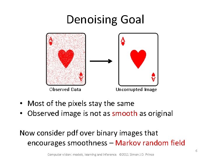
Denoising Goal Observed Data Uncorrupted Image • Most of the pixels stay the same • Observed image is not as smooth as original Now consider pdf over binary images that encourages smoothness – Markov random field Computer vision: models, learning and inference. © 2011 Simon J. D. Prince 6

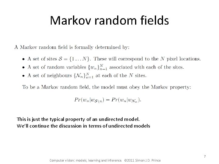
Markov random fields This is just the typical property of an undirected model. We’ll continue the discussion in terms of undirected models Computer vision: models, learning and inference. © 2011 Simon J. D. Prince 7

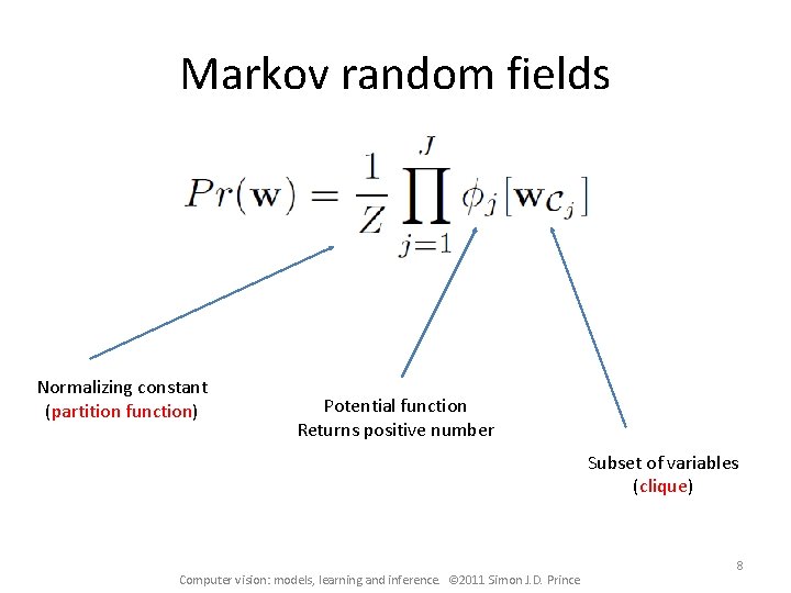
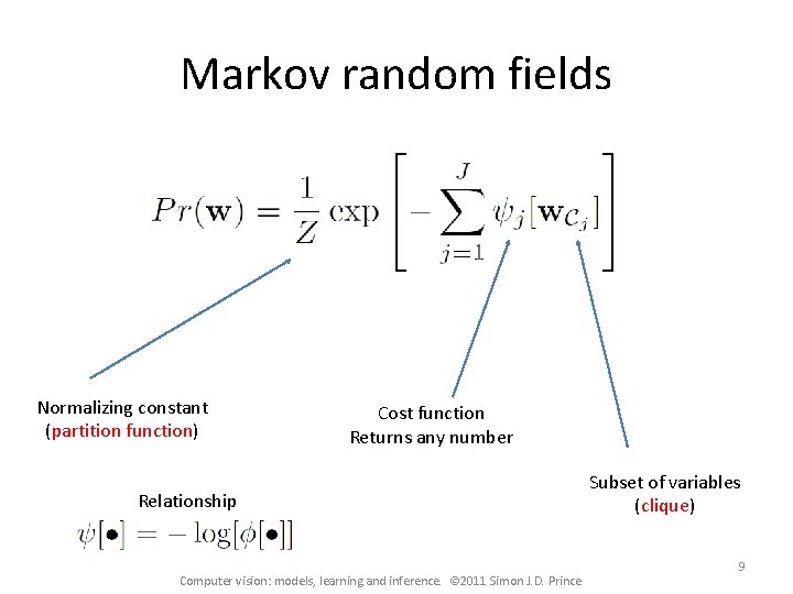
Markov random fields Normalizing constant (partition function) Potential function Returns positive number Subset of variables (clique) Computer vision: models, learning and inference. © 2011 Simon J. D. Prince 8

Markov random fields Normalizing constant (partition function) Cost function Returns any number Relationship Computer vision: models, learning and inference. © 2011 Simon J. D. Prince Subset of variables (clique) 9

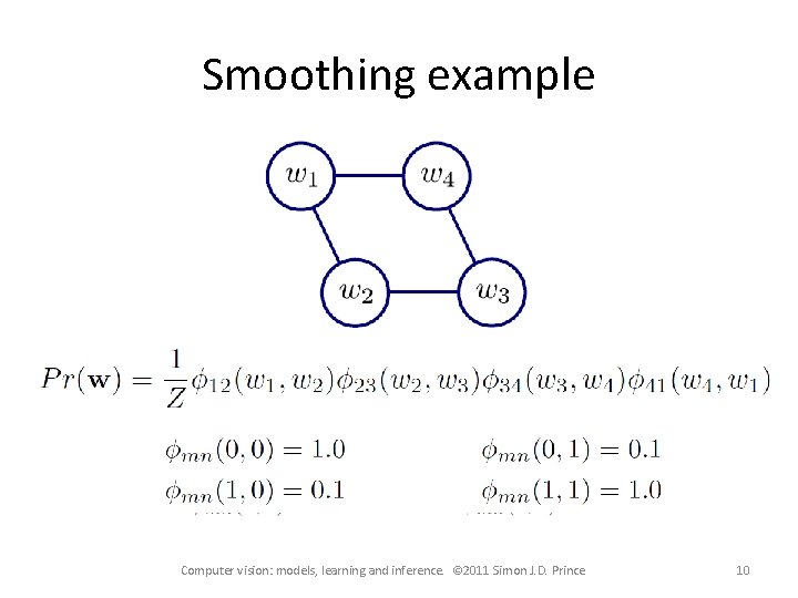
Smoothing example Computer vision: models, learning and inference. © 2011 Simon J. D. Prince 10

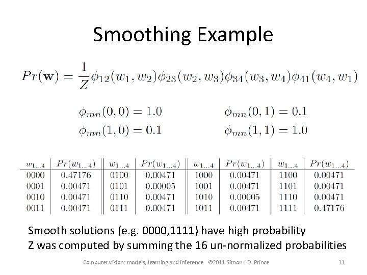
Smoothing Example Smooth solutions (e. g. 0000, 1111) have high probability Z was computed by summing the 16 un-normalized probabilities Computer vision: models, learning and inference. © 2011 Simon J. D. Prince 11

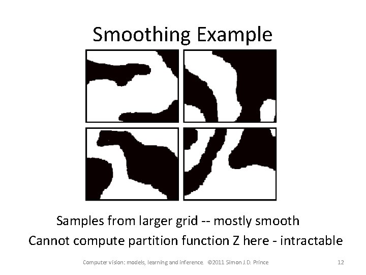
Smoothing Example Samples from larger grid -- mostly smooth Cannot compute partition function Z here - intractable Computer vision: models, learning and inference. © 2011 Simon J. D. Prince 12

Denoising Goal Observed Data Uncorrupted Image Computer vision: models, learning and inference. © 2011 Simon J. D. Prince 13

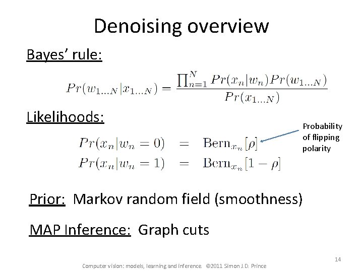
Denoising overview Bayes’ rule: Likelihoods: Probability of flipping polarity Prior: Markov random field (smoothness) MAP Inference: Graph cuts Computer vision: models, learning and inference. © 2011 Simon J. D. Prince 14

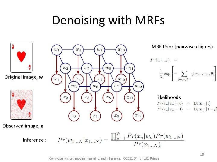
Denoising with MRFs MRF Prior (pairwise cliques) Original image, w Likelihoods Observed image, x Inference : Computer vision: models, learning and inference. © 2011 Simon J. D. Prince 15

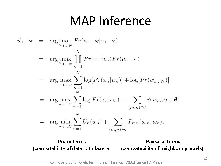
MAP Inference Unary terms (compatability of data with label y) Pairwise terms (compatability of neighboring labels) Computer vision: models, learning and inference. © 2011 Simon J. D. Prince 16

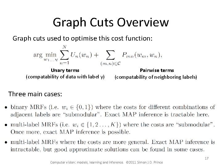
Graph Cuts Overview Graph cuts used to optimise this cost function: Unary terms (compatability of data with label y) Pairwise terms (compatability of neighboring labels) Three main cases: Computer vision: models, learning and inference. © 2011 Simon J. D. Prince 17

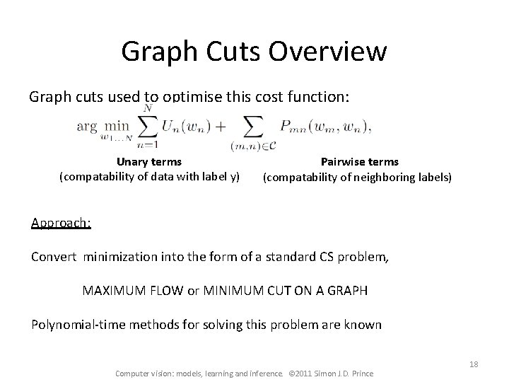
Graph Cuts Overview Graph cuts used to optimise this cost function: Unary terms (compatability of data with label y) Pairwise terms (compatability of neighboring labels) Approach: Convert minimization into the form of a standard CS problem, MAXIMUM FLOW or MINIMUM CUT ON A GRAPH Polynomial-time methods for solving this problem are known Computer vision: models, learning and inference. © 2011 Simon J. D. Prince 18

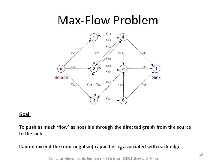
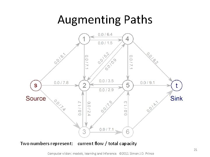
Max-Flow Problem Goal: To push as much ‘flow’ as possible through the directed graph from the source to the sink. Cannot exceed the (non-negative) capacities cij associated with each edge. Computer vision: models, learning and inference. © 2011 Simon J. D. Prince 19

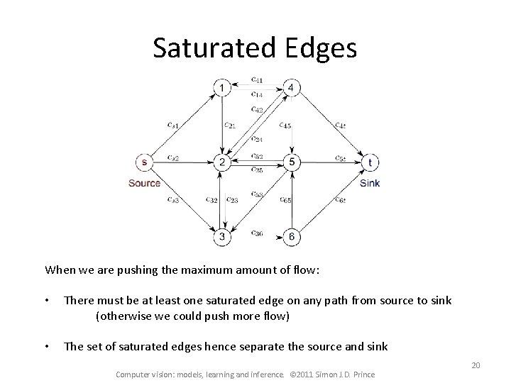
Saturated Edges When we are pushing the maximum amount of flow: • There must be at least one saturated edge on any path from source to sink (otherwise we could push more flow) • The set of saturated edges hence separate the source and sink Computer vision: models, learning and inference. © 2011 Simon J. D. Prince 20

Augmenting Paths Two numbers represent: current flow / total capacity Computer vision: models, learning and inference. © 2011 Simon J. D. Prince 21

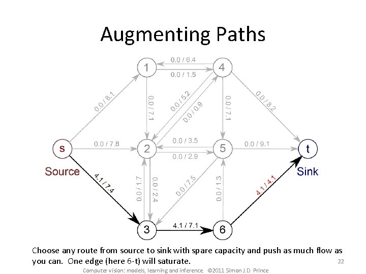
Augmenting Paths Choose any route from source to sink with spare capacity and push as much flow as 22 you can. One edge (here 6 -t) will saturate. Computer vision: models, learning and inference. © 2011 Simon J. D. Prince

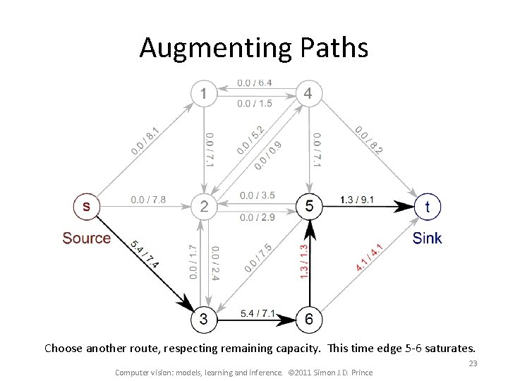
Augmenting Paths Choose another route, respecting remaining capacity. This time edge 5 -6 saturates. Computer vision: models, learning and inference. © 2011 Simon J. D. Prince 23

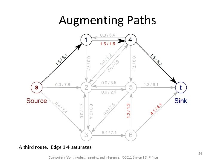
Augmenting Paths A third route. Edge 1 -4 saturates Computer vision: models, learning and inference. © 2011 Simon J. D. Prince 24

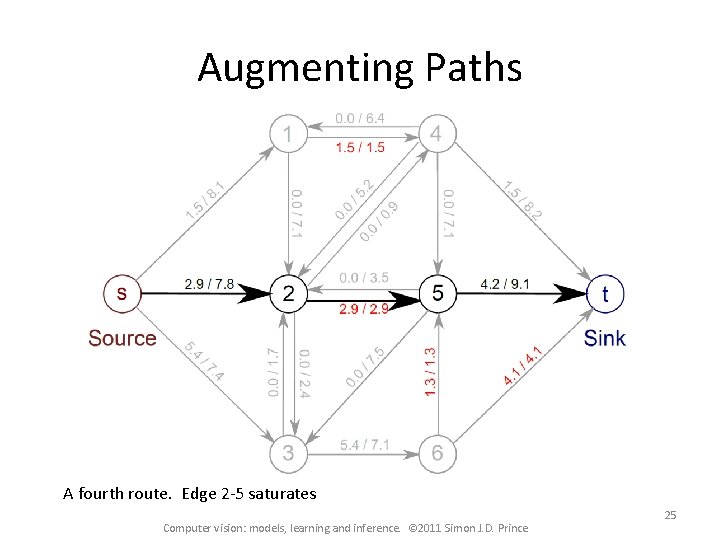
Augmenting Paths A fourth route. Edge 2 -5 saturates Computer vision: models, learning and inference. © 2011 Simon J. D. Prince 25

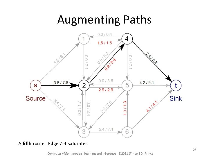
Augmenting Paths A fifth route. Edge 2 -4 saturates Computer vision: models, learning and inference. © 2011 Simon J. D. Prince 26

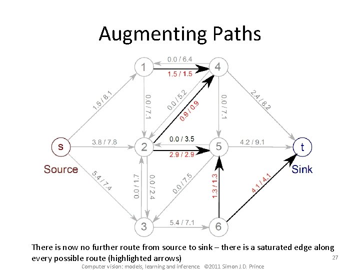
Augmenting Paths There is now no further route from source to sink – there is a saturated edge along 27 every possible route (highlighted arrows) Computer vision: models, learning and inference. © 2011 Simon J. D. Prince

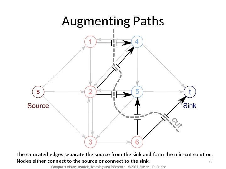
Augmenting Paths The saturated edges separate the source from the sink and form the min-cut solution. 28 Nodes either connect to the source or connect to the sink. Computer vision: models, learning and inference. © 2011 Simon J. D. Prince

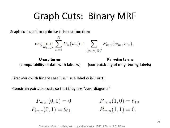
Graph Cuts: Binary MRF Graph cuts used to optimise this cost function: Unary terms (compatability of data with label w) Pairwise terms (compatability of neighboring labels) First work with binary case (i. e. True label w is 0 or 1) Constrain pairwise costs so that they are “zero-diagonal” 29 Computer vision: models, learning and inference. © 2011 Simon J. D. Prince

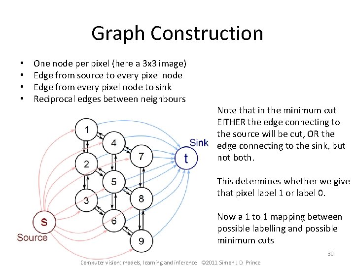
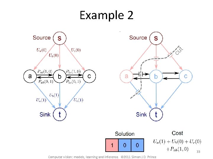
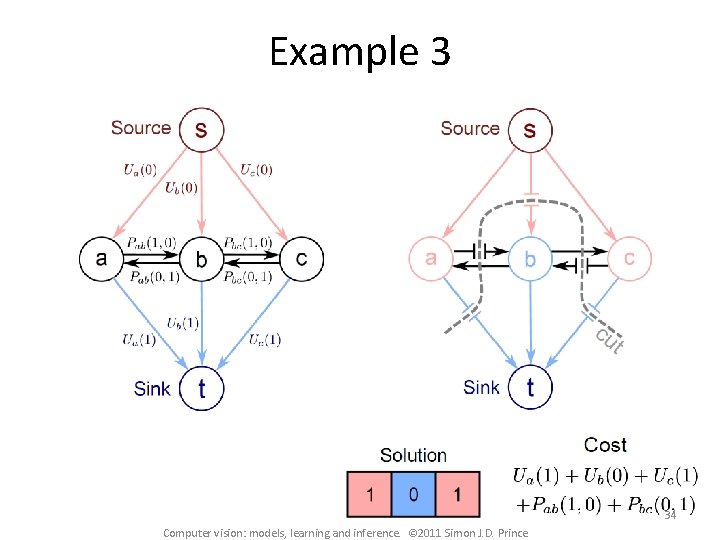
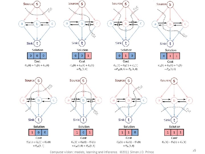
Graph Construction • • One node per pixel (here a 3 x 3 image) Edge from source to every pixel node Edge from every pixel node to sink Reciprocal edges between neighbours Note that in the minimum cut EITHER the edge connecting to the source will be cut, OR the edge connecting to the sink, but not both. This determines whether we give that pixel label 1 or label 0. Now a 1 to 1 mapping between possible labelling and possible minimum cuts 30 Computer vision: models, learning and inference. © 2011 Simon J. D. Prince

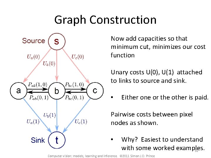
Graph Construction Now add capacities so that minimum cut, minimizes our cost function Unary costs U(0), U(1) attached to links to source and sink. • Either one or the other is paid. Pairwise costs between pixel nodes as shown. • Why? Easiest to understand with some worked examples. 31 Computer vision: models, learning and inference. © 2011 Simon J. D. Prince

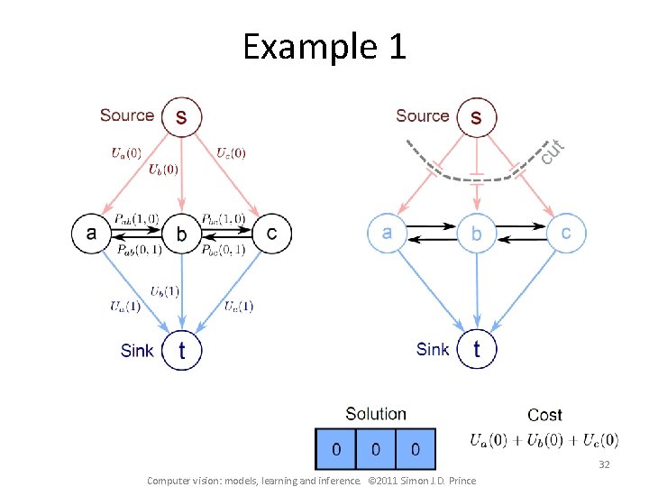
Example 1 32 Computer vision: models, learning and inference. © 2011 Simon J. D. Prince

Example 2 33 Computer vision: models, learning and inference. © 2011 Simon J. D. Prince

Example 3 34 Computer vision: models, learning and inference. © 2011 Simon J. D. Prince

Computer vision: models, learning and inference. © 2011 Simon J. D. Prince 35

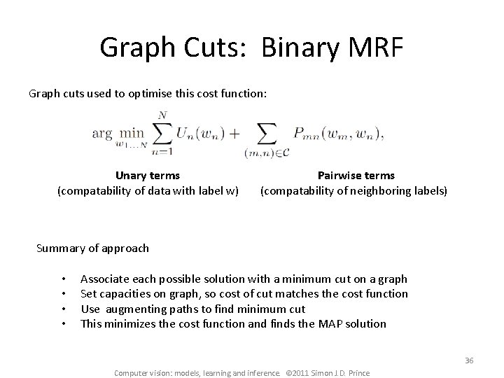
Graph Cuts: Binary MRF Graph cuts used to optimise this cost function: Unary terms (compatability of data with label w) Pairwise terms (compatability of neighboring labels) Summary of approach • • Associate each possible solution with a minimum cut on a graph Set capacities on graph, so cost of cut matches the cost function Use augmenting paths to find minimum cut This minimizes the cost function and finds the MAP solution 36 Computer vision: models, learning and inference. © 2011 Simon J. D. Prince

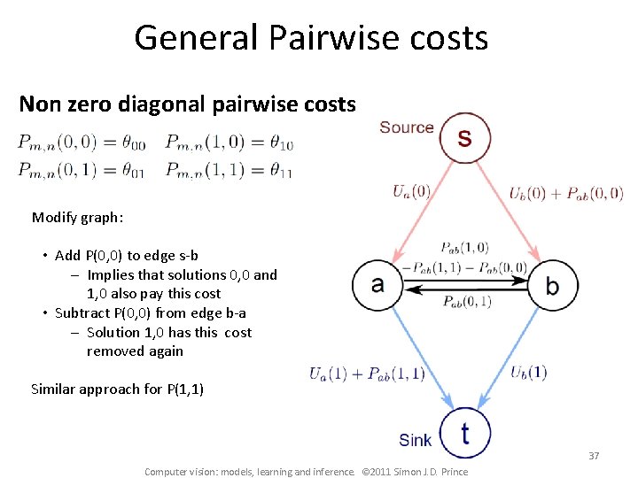
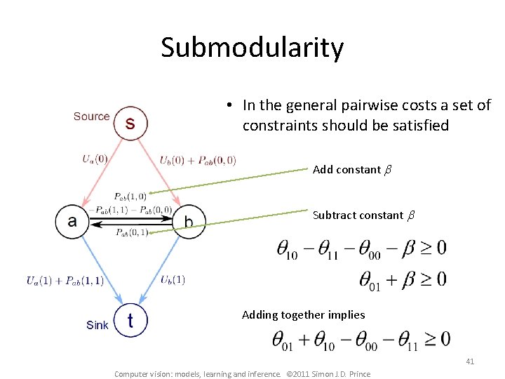
General Pairwise costs Non zero diagonal pairwise costs Modify graph: • Add P(0, 0) to edge s-b Implies that solutions 0, 0 and 1, 0 also pay this cost • Subtract P(0, 0) from edge b-a Solution 1, 0 has this cost removed again Similar approach for P(1, 1) 37 Computer vision: models, learning and inference. © 2011 Simon J. D. Prince

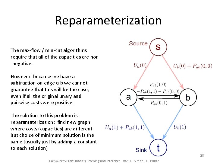
Reparameterization The max-flow / min-cut algorithms require that all of the capacities are non -negative. However, because we have a subtraction on edge a-b we cannot guarantee that this will be the case, even if all the original unary and pairwise costs were positive. The solution to this problem is reparamaterization: find new graph where costs (capacities) are different but choice of minimum solution is the same (usually just by adding a constant to each solution) 38 Computer vision: models, learning and inference. © 2011 Simon J. D. Prince

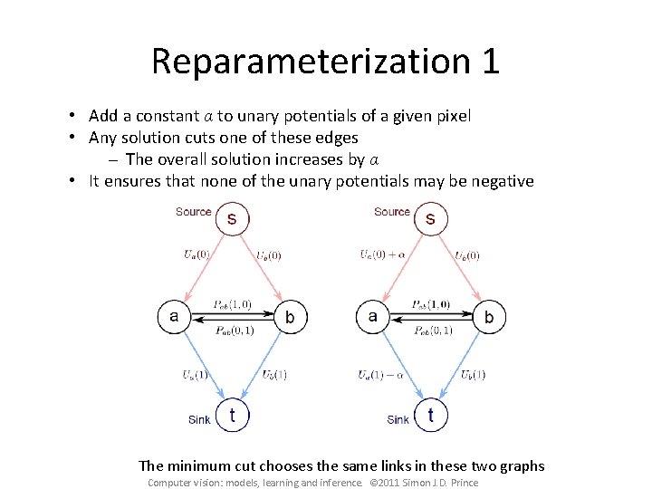
Reparameterization 1 • Add a constant α to unary potentials of a given pixel • Any solution cuts one of these edges The overall solution increases by α • It ensures that none of the unary potentials may be negative The minimum cut chooses the same links in these two graphs Computer vision: models, learning and inference. © 2011 Simon J. D. Prince

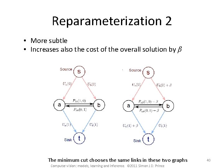
Reparameterization 2 • More subtle • Increases also the cost of the overall solution by β The minimum cut chooses the same links in these two graphs Computer vision: models, learning and inference. © 2011 Simon J. D. Prince 40

Submodularity • In the general pairwise costs a set of constraints should be satisfied Add constant b Subtract constant b Adding together implies 41 Computer vision: models, learning and inference. © 2011 Simon J. D. Prince

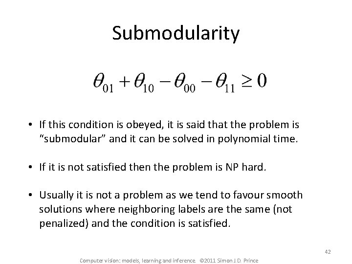
Submodularity • If this condition is obeyed, it is said that the problem is “submodular” and it can be solved in polynomial time. • If it is not satisfied then the problem is NP hard. • Usually it is not a problem as we tend to favour smooth solutions where neighboring labels are the same (not penalized) and the condition is satisfied. 42 Computer vision: models, learning and inference. © 2011 Simon J. D. Prince

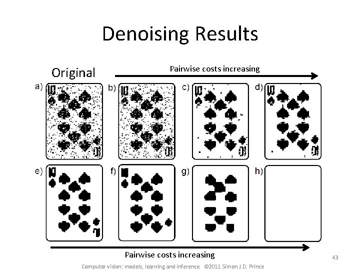
Denoising Results Original Pairwise costs increasing Computer vision: models, learning and inference. © 2011 Simon J. D. Prince 43

Plan of Talk • • • Denoising problem Markov random fields (MRFs) Max-flow / min-cut Binary MRFs – submodular (exact solution) Multi-label MRFs - non-submodular (approximate) 44 Computer vision: models, learning and inference. © 2011 Simon J. D. Prince

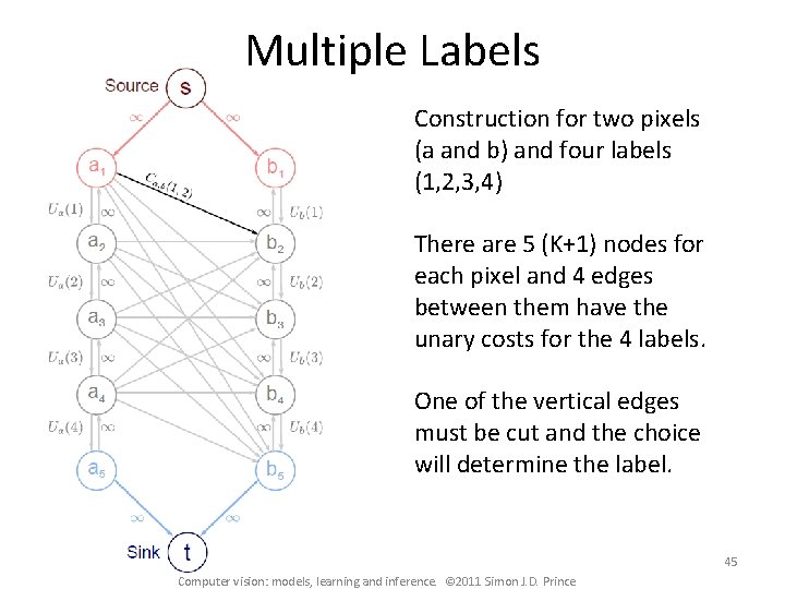
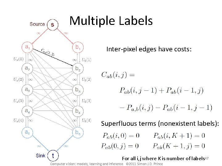
Multiple Labels Construction for two pixels (a and b) and four labels (1, 2, 3, 4) There are 5 (K+1) nodes for each pixel and 4 edges between them have the unary costs for the 4 labels. One of the vertical edges must be cut and the choice will determine the label. 45 Computer vision: models, learning and inference. © 2011 Simon J. D. Prince

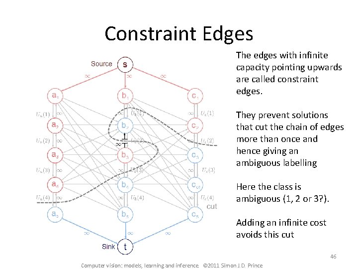
Constraint Edges The edges with infinite capacity pointing upwards are called constraint edges. They prevent solutions that cut the chain of edges more than once and hence giving an ambiguous labelling Here the class is ambiguous (1, 2 or 3? ). Adding an infinite cost avoids this cut 46 Computer vision: models, learning and inference. © 2011 Simon J. D. Prince

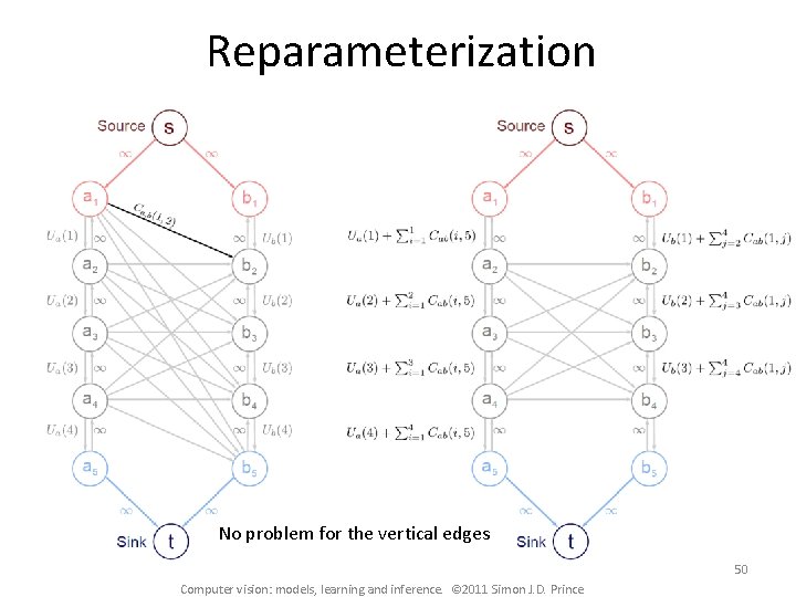
Multiple Labels Inter-pixel edges have costs: Superfluous terms (nonexistent labels): For all i, j where K is number of labels 47 Computer vision: models, learning and inference. © 2011 Simon J. D. Prince

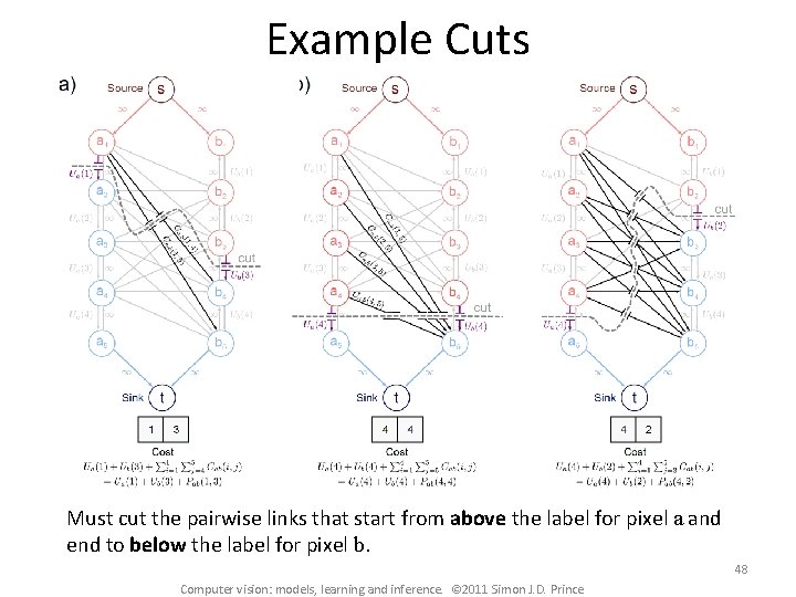
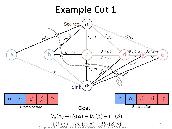
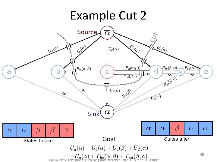
Example Cuts Must cut the pairwise links that start from above the label for pixel a and end to below the label for pixel b. 48 Computer vision: models, learning and inference. © 2011 Simon J. D. Prince

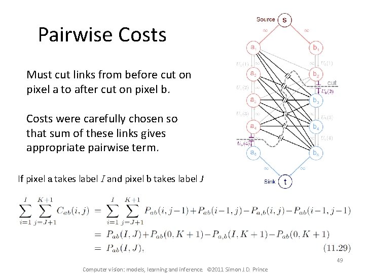
Pairwise Costs Must cut links from before cut on pixel a to after cut on pixel b. Costs were carefully chosen so that sum of these links gives appropriate pairwise term. If pixel a takes label I and pixel b takes label J 49 Computer vision: models, learning and inference. © 2011 Simon J. D. Prince

Reparameterization No problem for the vertical edges 50 Computer vision: models, learning and inference. © 2011 Simon J. D. Prince

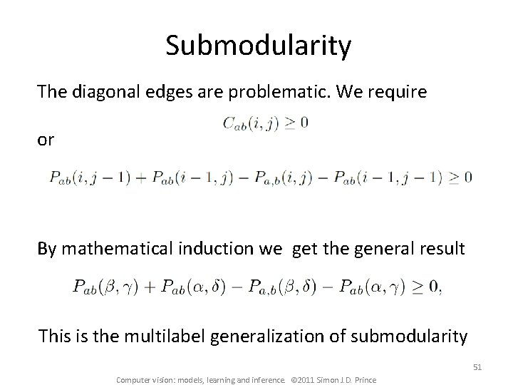
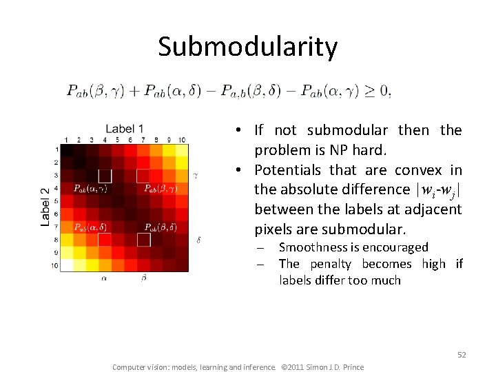
Submodularity The diagonal edges are problematic. We require or By mathematical induction we get the general result This is the multilabel generalization of submodularity 51 Computer vision: models, learning and inference. © 2011 Simon J. D. Prince

Submodularity • If not submodular then the problem is NP hard. • Potentials that are convex in the absolute difference |wi-wj| between the labels at adjacent pixels are submodular. Smoothness is encouraged The penalty becomes high if labels differ too much 52 Computer vision: models, learning and inference. © 2011 Simon J. D. Prince

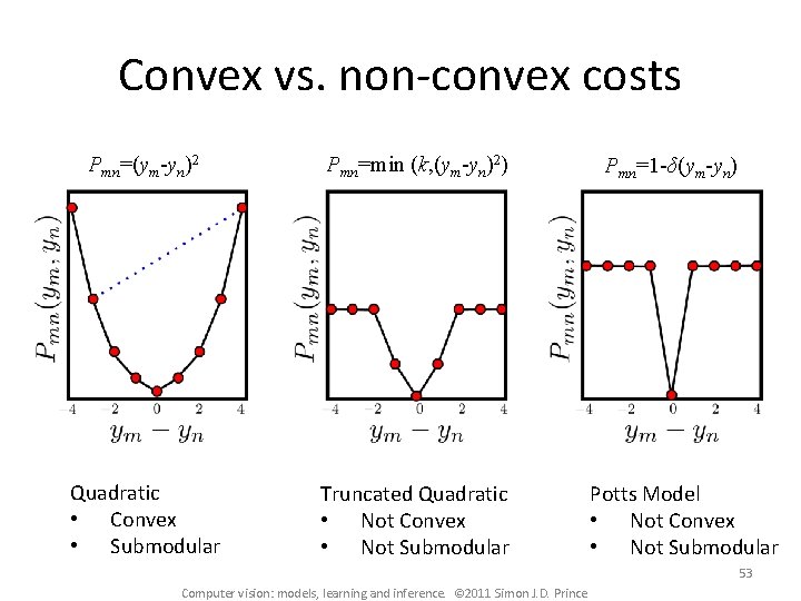
Convex vs. non-convex costs Pmn=(ym-yn)2 Pmn=min (k, (ym-yn)2) Quadratic • Convex • Submodular Truncated Quadratic • Not Convex • Not Submodular Pmn=1 -δ(ym-yn) Potts Model • Not Convex • Not Submodular 53 Computer vision: models, learning and inference. © 2011 Simon J. D. Prince

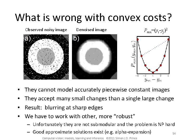
What is wrong with convex costs? Observed noisy image • • Denoised image Pmn=(yi-yj)2 They cannot model accurately piecewise constant images They accept many small changes than a single large change Result: blurring at sharp edges We have to work with other, more “robust” – Unfortunately they are not submodular and the problem is NP hard – Good approximate solutions exist (e. g. alpha-expansion) 54 Computer vision: models, learning and inference. © 2011 Simon J. D. Prince

Plan of Talk • • • Denoising problem Markov random fields (MRFs) Max-flow / min-cut Binary MRFs - submodular (exact solution) Multi-label MRFs – submodular (exact solution) Multi-label MRFs - non-submodular (approximate) 55 Computer vision: models, learning and inference. © 2011 Simon J. D. Prince

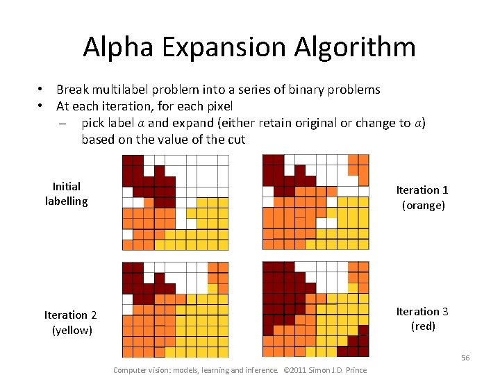
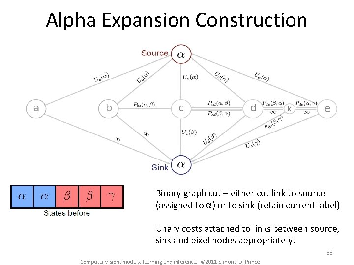
Alpha Expansion Algorithm • Break multilabel problem into a series of binary problems • At each iteration, for each pixel pick label α and expand (either retain original or change to α) based on the value of the cut Initial labelling Iteration 1 (orange) Iteration 2 (yellow) Iteration 3 (red) 56 Computer vision: models, learning and inference. © 2011 Simon J. D. Prince

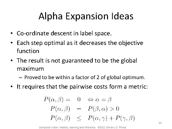
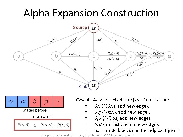
Alpha Expansion Ideas • Co-ordinate descent in label space. • Each step optimal as it decreases the objective function • The result is not guaranteed to be the global maximum – Proved to be within a factor of 2 of global optimum. • It requires that the pairwise costs form a metric: 57 Computer vision: models, learning and inference. © 2011 Simon J. D. Prince

Alpha Expansion Construction Binary graph cut – either cut link to source (assigned to a) or to sink (retain current label) Unary costs attached to links between source, sink and pixel nodes appropriately. 58 Computer vision: models, learning and inference. © 2011 Simon J. D. Prince

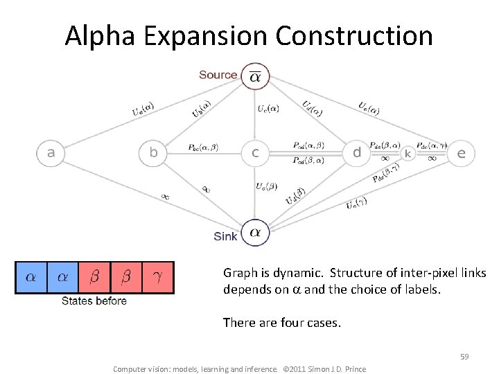
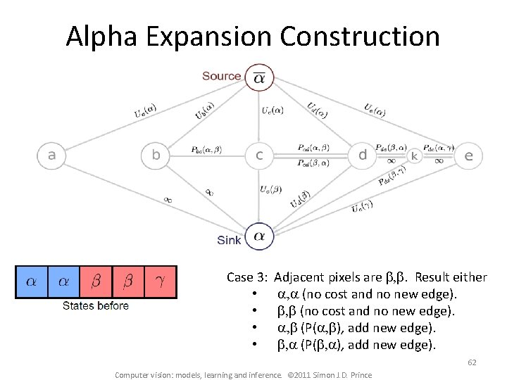
Alpha Expansion Construction Graph is dynamic. Structure of inter-pixel links depends on a and the choice of labels. There are four cases. 59 Computer vision: models, learning and inference. © 2011 Simon J. D. Prince

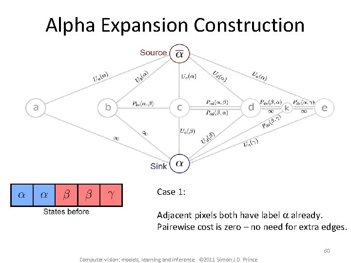
Alpha Expansion Construction Case 1: Adjacent pixels both have label a already. Pairewise cost is zero – no need for extra edges. 60 Computer vision: models, learning and inference. © 2011 Simon J. D. Prince

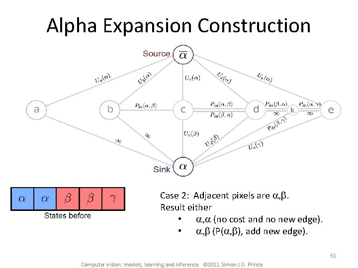
Alpha Expansion Construction Case 2: Adjacent pixels are a, b. Result either • a, a (no cost and no new edge). • a, b (P(a, b), add new edge). 61 Computer vision: models, learning and inference. © 2011 Simon J. D. Prince

Alpha Expansion Construction Case 3: • • Adjacent pixels are b, b. Result either a, a (no cost and no new edge). b, b (no cost and no new edge). a, b (P(a, b), add new edge). b, a (P(b, a), add new edge). 62 Computer vision: models, learning and inference. © 2011 Simon J. D. Prince

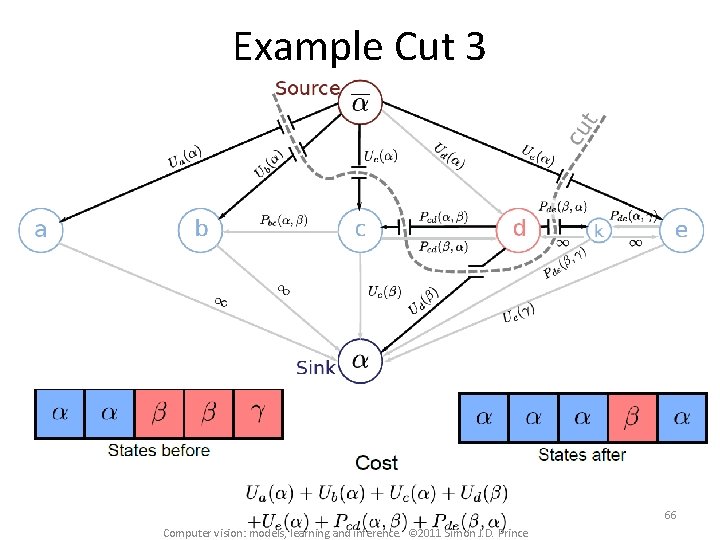
Alpha Expansion Construction Important! Case 4: • • • Adjacent pixels are b, g. Result either b, g (P(b, g), add new edge). a, g (P(a, g), add new edge). b, a (P(b, a), add new edge). a, a (no cost and no new edge). 63 extra node k between the adjacent pixels Computer vision: models, learning and inference. © 2011 Simon J. D. Prince

Example Cut 1 64 Computer vision: models, learning and inference. © 2011 Simon J. D. Prince

Example Cut 2 65 Computer vision: models, learning and inference. © 2011 Simon J. D. Prince

Example Cut 3 66 Computer vision: models, learning and inference. © 2011 Simon J. D. Prince

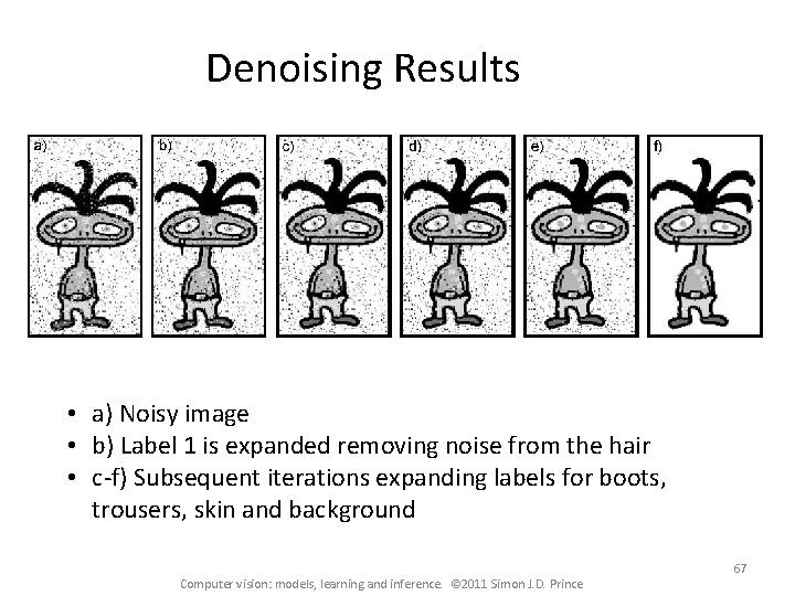
Denoising Results • a) Noisy image • b) Label 1 is expanded removing noise from the hair • c-f) Subsequent iterations expanding labels for boots, trousers, skin and background Computer vision: models, learning and inference. © 2011 Simon J. D. Prince 67

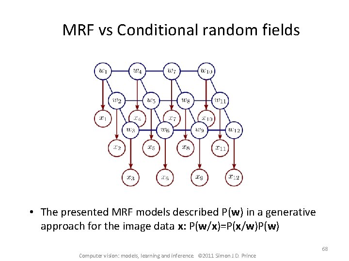
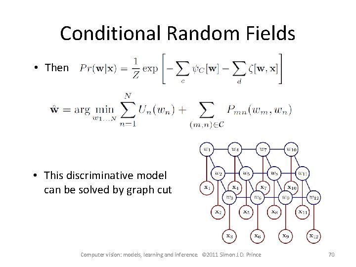
MRF vs Conditional random fields • The presented MRF models described P(w) in a generative approach for the image data x: P(w/x)=P(x/w)P(w) Computer vision: models, learning and inference. © 2011 Simon J. D. Prince 68

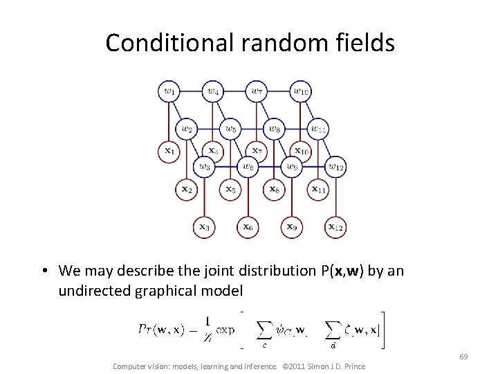
Conditional random fields • We may describe the joint distribution P(x, w) by an undirected graphical model Computer vision: models, learning and inference. © 2011 Simon J. D. Prince 69

Conditional Random Fields • Then • This discriminative model can be solved by graph cut Computer vision: models, learning and inference. © 2011 Simon J. D. Prince 70

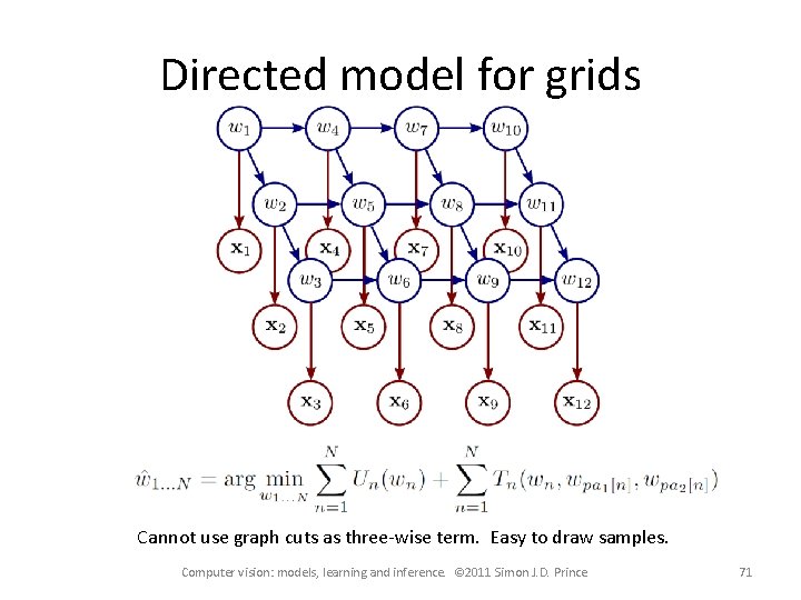
Directed model for grids Cannot use graph cuts as three-wise term. Easy to draw samples. Computer vision: models, learning and inference. © 2011 Simon J. D. Prince 71

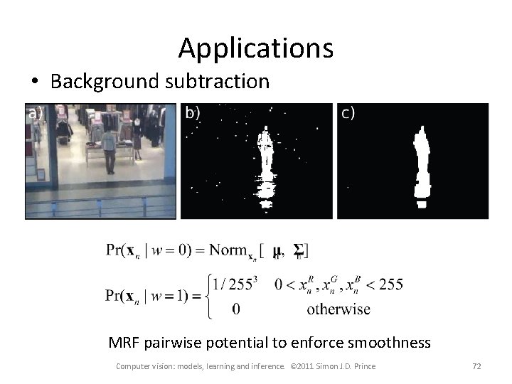
Applications • Background subtraction MRF pairwise potential to enforce smoothness Computer vision: models, learning and inference. © 2011 Simon J. D. Prince 72

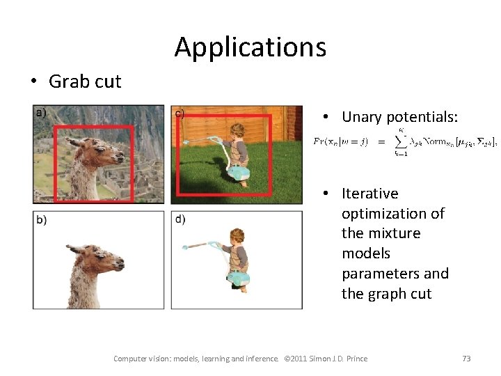
Applications • Grab cut • Unary potentials: • Iterative optimization of the mixture models parameters and the graph cut Computer vision: models, learning and inference. © 2011 Simon J. D. Prince 73

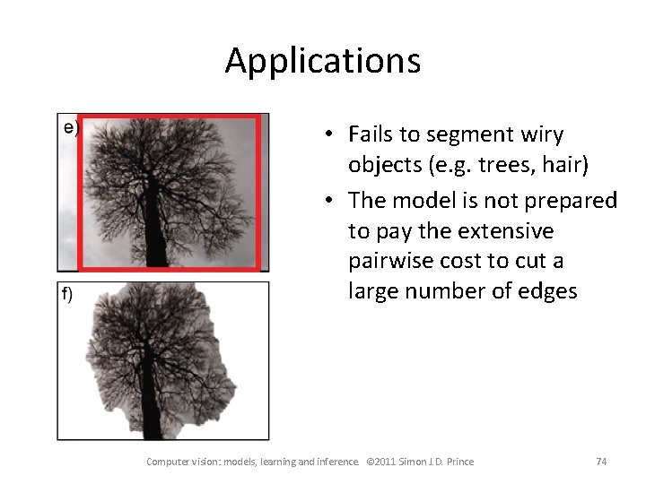
Applications • Fails to segment wiry objects (e. g. trees, hair) • The model is not prepared to pay the extensive pairwise cost to cut a large number of edges Computer vision: models, learning and inference. © 2011 Simon J. D. Prince 74

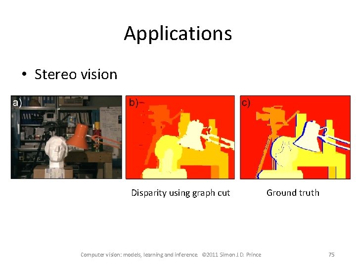
Applications • Stereo vision Disparity using graph cut Computer vision: models, learning and inference. © 2011 Simon J. D. Prince Ground truth 75

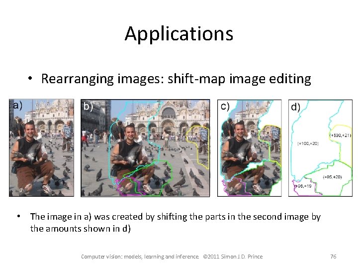
Applications • Rearranging images: shift-map image editing • The image in a) was created by shifting the parts in the second image by the amounts shown in d) Computer vision: models, learning and inference. © 2011 Simon J. D. Prince 76

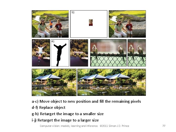
a-c) Move object to new position and fill the remaining pixels d-f) Replace object g-h) Retarget the image to a smaller size i-j) Retarget the image to a larger size Computer vision: models, learning and inference. © 2011 Simon J. D. Prince 77

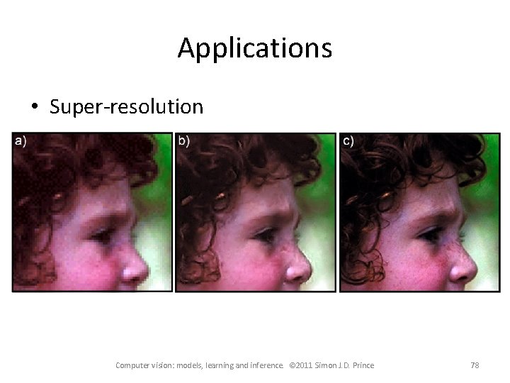
Applications • Super-resolution Computer vision: models, learning and inference. © 2011 Simon J. D. Prince 78

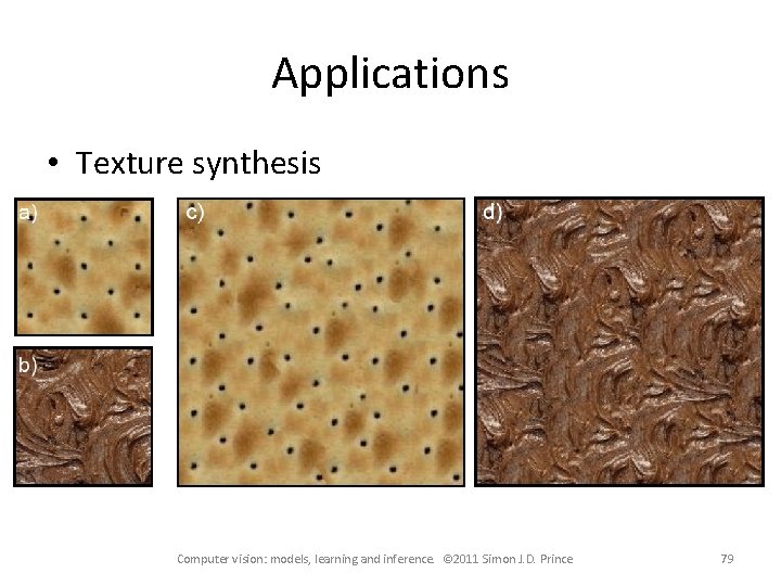
Applications • Texture synthesis Computer vision: models, learning and inference. © 2011 Simon J. D. Prince 79

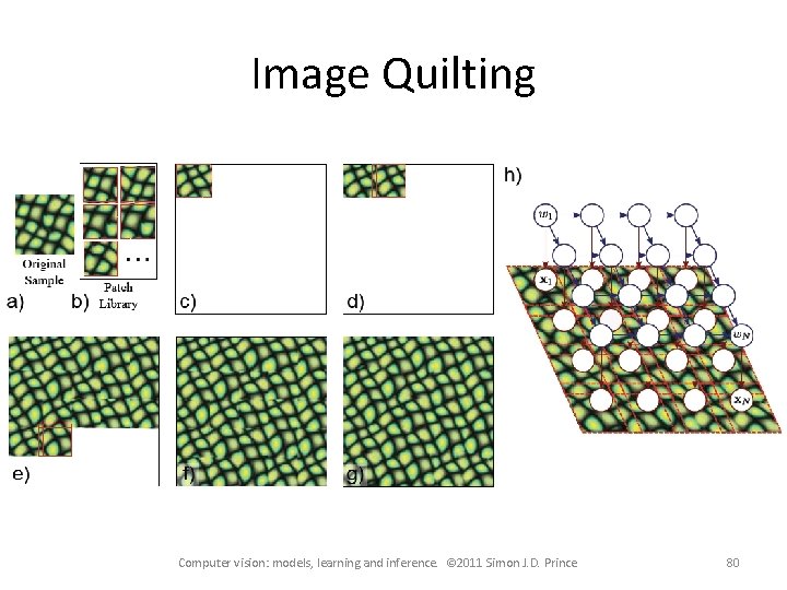
Image Quilting Computer vision: models, learning and inference. © 2011 Simon J. D. Prince 80

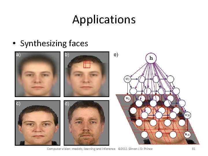
Applications • Synthesizing faces Computer vision: models, learning and inference. © 2011 Simon J. D. Prince 81