Computer vision models learning and inference Chapter 4

Computer vision: models, learning and inference Chapter 4 Fitting probability models Please send errata to s. prince@cs. ucl. ac. uk

Structure • Fitting probability distributions – Maximum likelihood – Maximum a posteriori – Bayesian approach • Worked example 1: Normal distribution • Worked example 2: Categorical distribution Computer vision: models, learning and inference. © 2011 Simon J. D. Prince 2

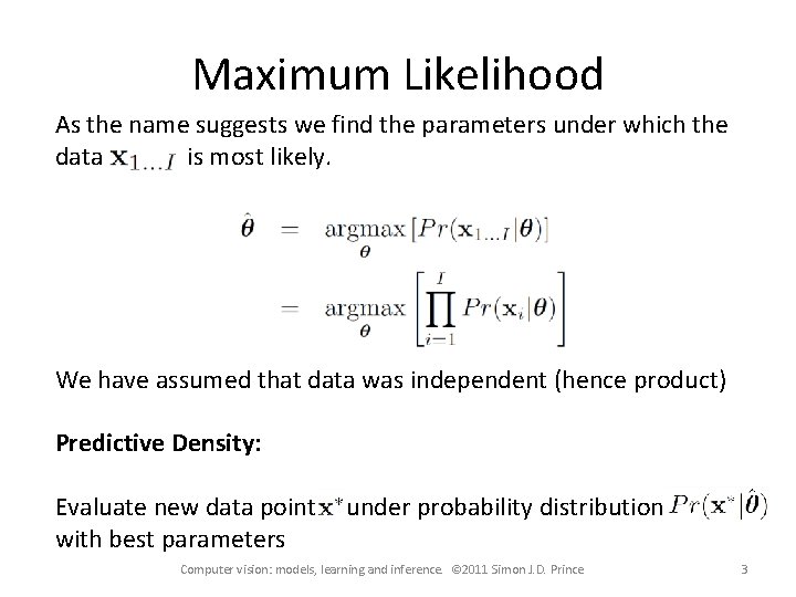
Maximum Likelihood As the name suggests we find the parameters under which the data is most likely. We have assumed that data was independent (hence product) Predictive Density: Evaluate new data point with best parameters under probability distribution Computer vision: models, learning and inference. © 2011 Simon J. D. Prince 3

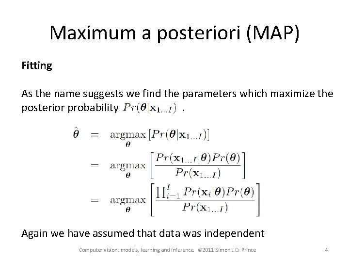
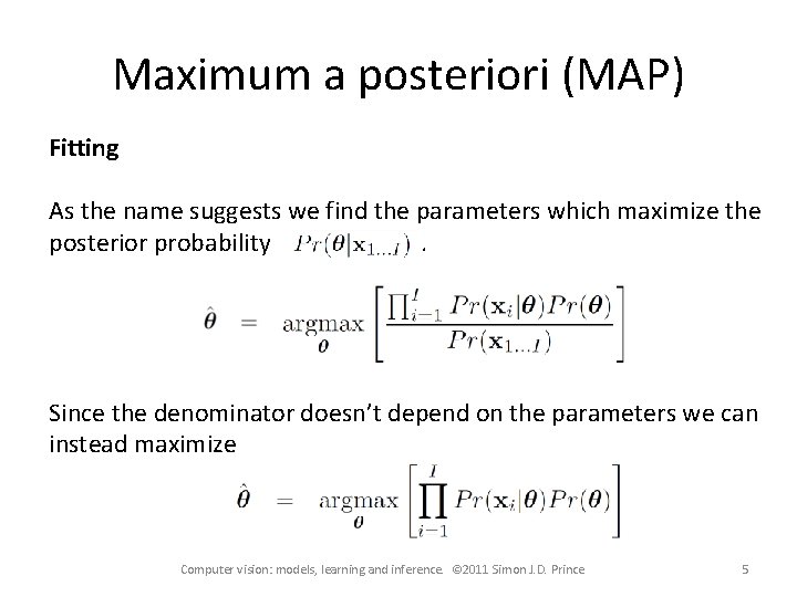
Maximum a posteriori (MAP) Fitting As the name suggests we find the parameters which maximize the posterior probability. Again we have assumed that data was independent Computer vision: models, learning and inference. © 2011 Simon J. D. Prince 4

Maximum a posteriori (MAP) Fitting As the name suggests we find the parameters which maximize the posterior probability. Since the denominator doesn’t depend on the parameters we can instead maximize Computer vision: models, learning and inference. © 2011 Simon J. D. Prince 5

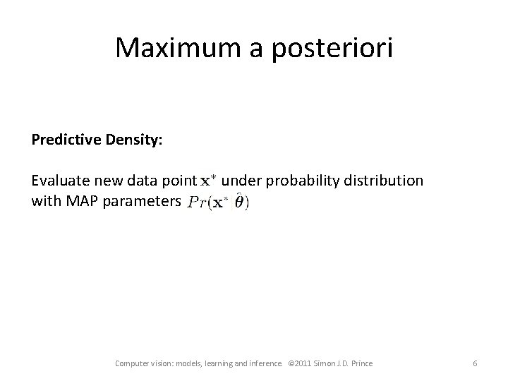
Maximum a posteriori Predictive Density: Evaluate new data point with MAP parameters under probability distribution Computer vision: models, learning and inference. © 2011 Simon J. D. Prince 6

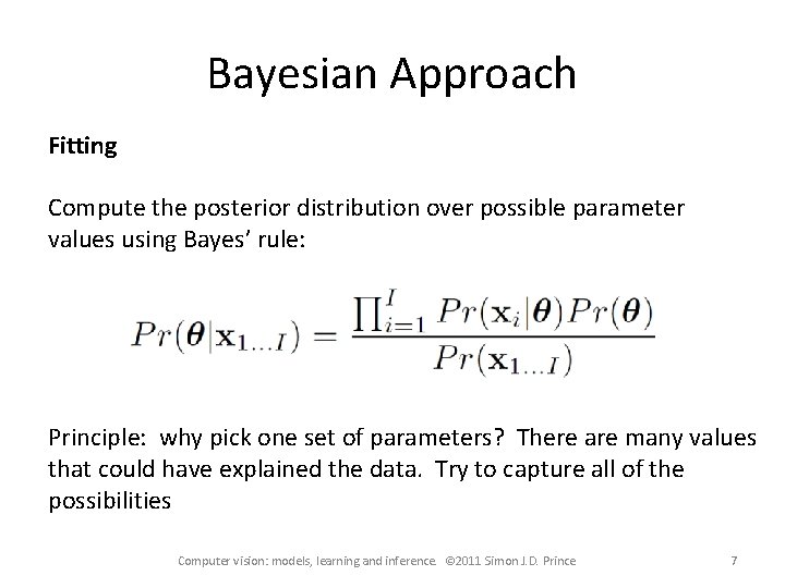
Bayesian Approach Fitting Compute the posterior distribution over possible parameter values using Bayes’ rule: Principle: why pick one set of parameters? There are many values that could have explained the data. Try to capture all of the possibilities Computer vision: models, learning and inference. © 2011 Simon J. D. Prince 7

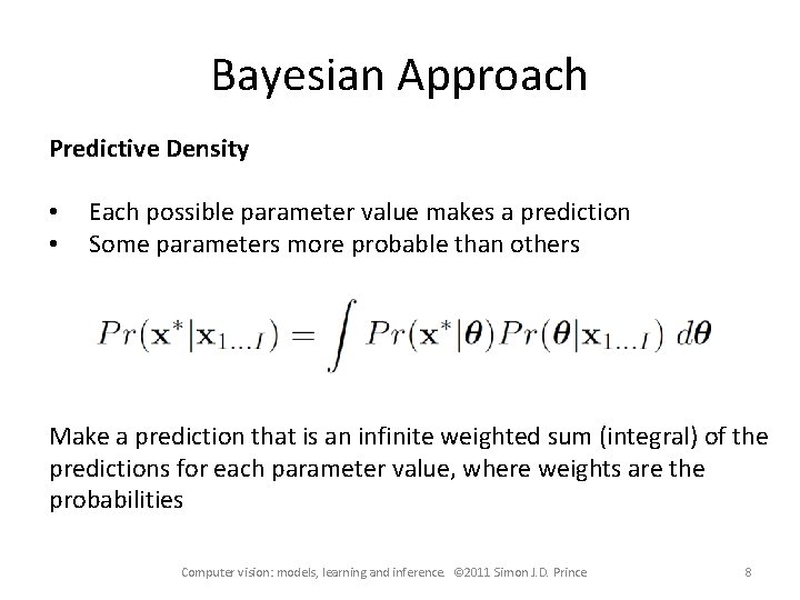
Bayesian Approach Predictive Density • • Each possible parameter value makes a prediction Some parameters more probable than others Make a prediction that is an infinite weighted sum (integral) of the predictions for each parameter value, where weights are the probabilities Computer vision: models, learning and inference. © 2011 Simon J. D. Prince 8

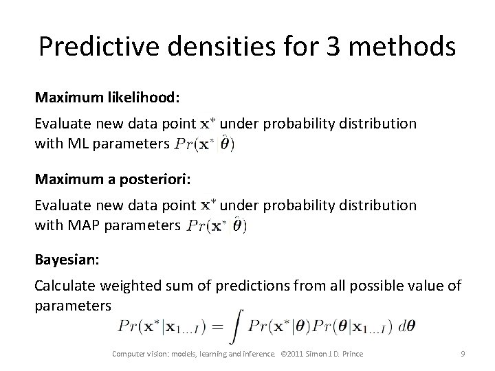
Predictive densities for 3 methods Maximum likelihood: Evaluate new data point with ML parameters under probability distribution Maximum a posteriori: Evaluate new data point with MAP parameters under probability distribution Bayesian: Calculate weighted sum of predictions from all possible value of parameters Computer vision: models, learning and inference. © 2011 Simon J. D. Prince 9

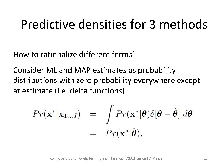
Predictive densities for 3 methods How to rationalize different forms? Consider ML and MAP estimates as probability distributions with zero probability everywhere except at estimate (i. e. delta functions) Computer vision: models, learning and inference. © 2011 Simon J. D. Prince 10

Structure • Fitting probability distributions – Maximum likelihood – Maximum a posteriori – Bayesian approach • Worked example 1: Normal distribution • Worked example 2: Categorical distribution Computer vision: models, learning and inference. © 2011 Simon J. D. Prince 11

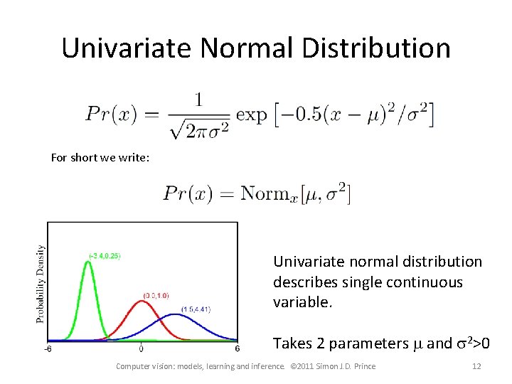
Univariate Normal Distribution For short we write: Univariate normal distribution describes single continuous variable. Takes 2 parameters m and s 2>0 Computer vision: models, learning and inference. © 2011 Simon J. D. Prince 12

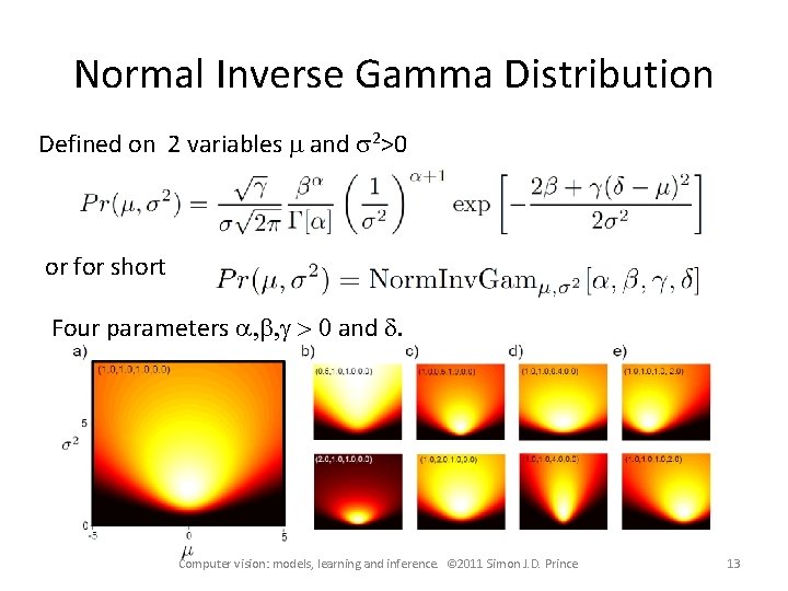
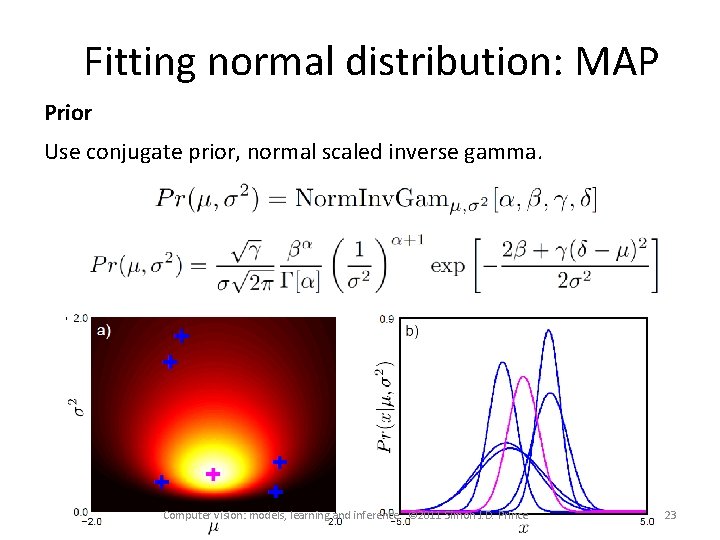
Normal Inverse Gamma Distribution Defined on 2 variables m and s 2>0 or for short Four parameters a, b, g > 0 and d. Computer vision: models, learning and inference. © 2011 Simon J. D. Prince 13

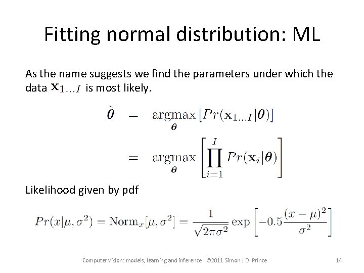
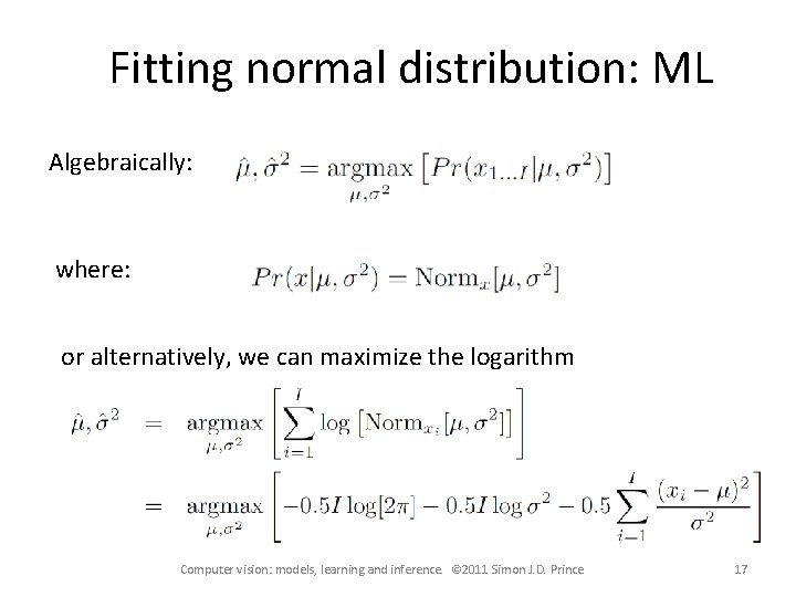
Fitting normal distribution: ML As the name suggests we find the parameters under which the data is most likely. Likelihood given by pdf Computer vision: models, learning and inference. © 2011 Simon J. D. Prince 14

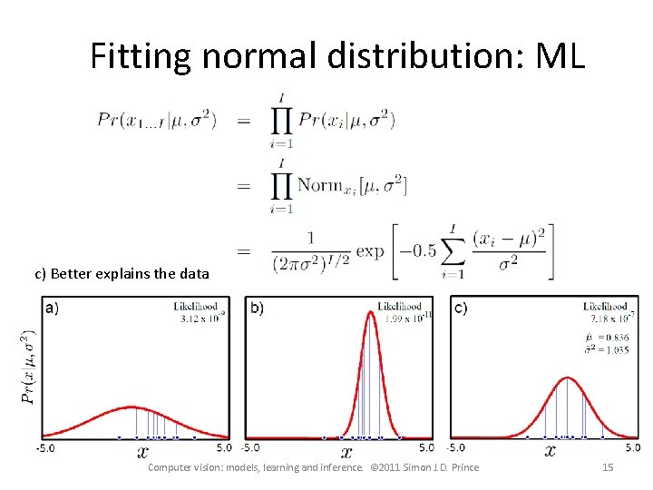
Fitting normal distribution: ML c) Better explains the data Computer vision: models, learning and inference. © 2011 Simon J. D. Prince 15

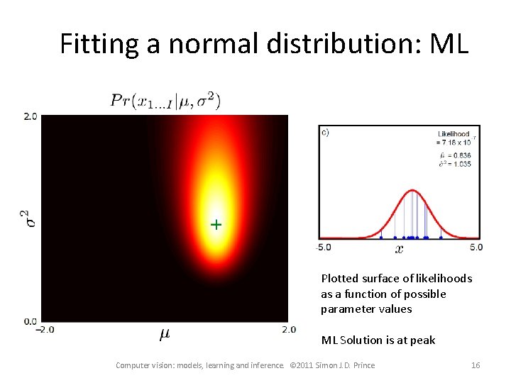
Fitting a normal distribution: ML Plotted surface of likelihoods as a function of possible parameter values ML Solution is at peak Computer vision: models, learning and inference. © 2011 Simon J. D. Prince 16

Fitting normal distribution: ML Algebraically: where: or alternatively, we can maximize the logarithm Computer vision: models, learning and inference. © 2011 Simon J. D. Prince 17

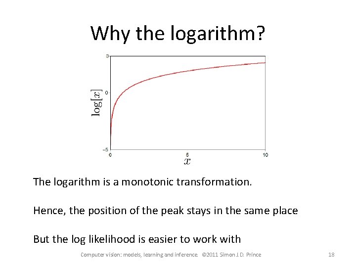
Why the logarithm? The logarithm is a monotonic transformation. Hence, the position of the peak stays in the same place But the log likelihood is easier to work with Computer vision: models, learning and inference. © 2011 Simon J. D. Prince 18

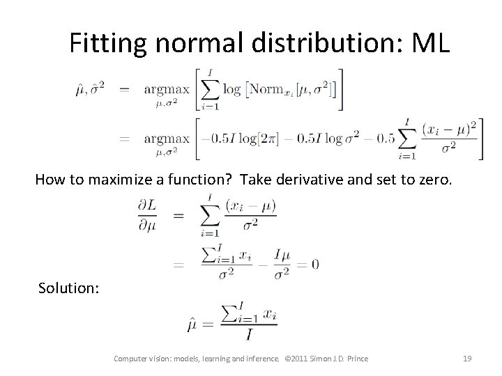
Fitting normal distribution: ML How to maximize a function? Take derivative and set to zero. Solution: Computer vision: models, learning and inference. © 2011 Simon J. D. Prince 19

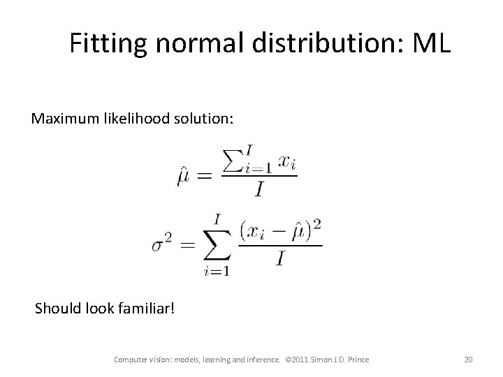
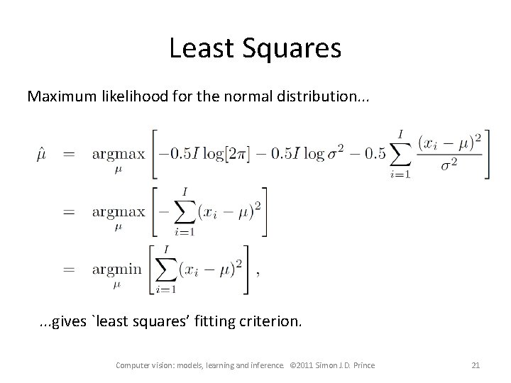
Fitting normal distribution: ML Maximum likelihood solution: Should look familiar! Computer vision: models, learning and inference. © 2011 Simon J. D. Prince 20

Least Squares Maximum likelihood for the normal distribution. . . gives `least squares’ fitting criterion. Computer vision: models, learning and inference. © 2011 Simon J. D. Prince 21

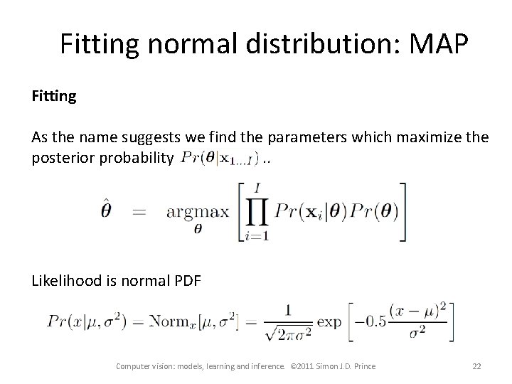
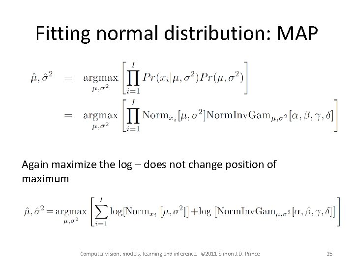
Fitting normal distribution: MAP Fitting As the name suggests we find the parameters which maximize the posterior probability. . Likelihood is normal PDF Computer vision: models, learning and inference. © 2011 Simon J. D. Prince 22

Fitting normal distribution: MAP Prior Use conjugate prior, normal scaled inverse gamma. Computer vision: models, learning and inference. © 2011 Simon J. D. Prince 23

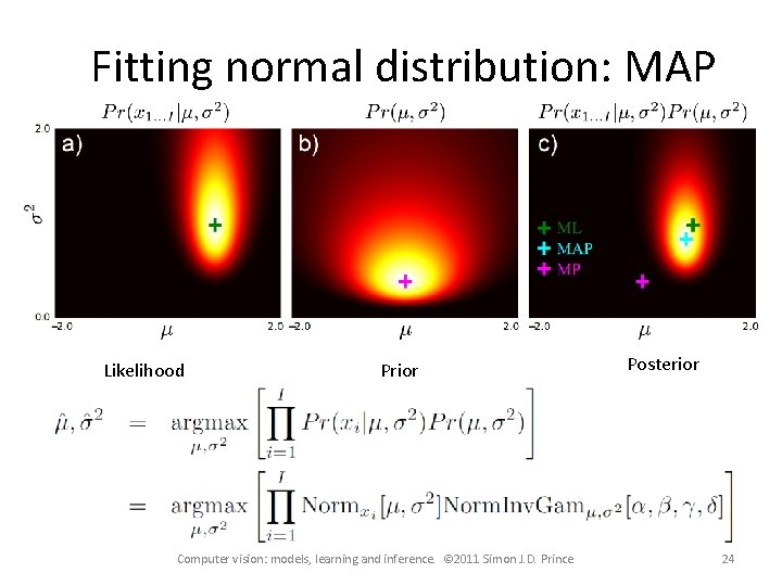
Fitting normal distribution: MAP Likelihood Prior Computer vision: models, learning and inference. © 2011 Simon J. D. Prince Posterior 24

Fitting normal distribution: MAP Again maximize the log – does not change position of maximum Computer vision: models, learning and inference. © 2011 Simon J. D. Prince 25

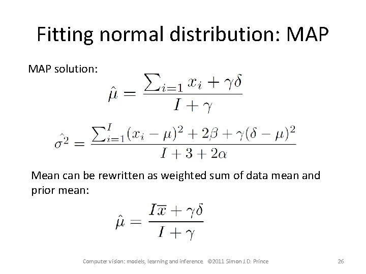
Fitting normal distribution: MAP solution: Mean can be rewritten as weighted sum of data mean and prior mean: Computer vision: models, learning and inference. © 2011 Simon J. D. Prince 26

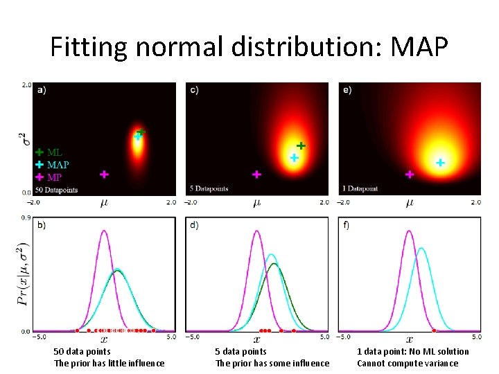
Fitting normal distribution: MAP 50 data points The prior has little influence 5 data points The prior has some influence 1 data point: No ML solution Cannot compute variance

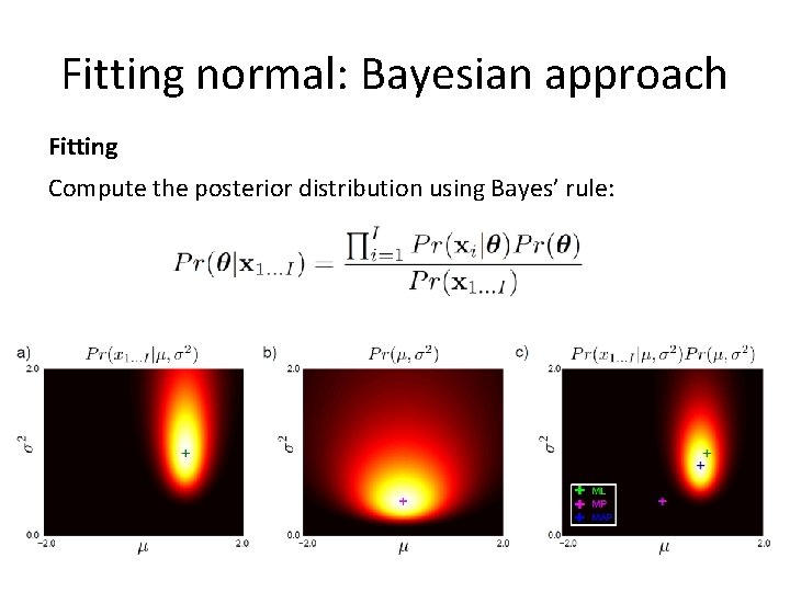
Fitting normal: Bayesian approach Fitting Compute the posterior distribution using Bayes’ rule:

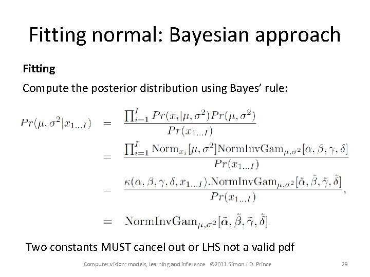
Fitting normal: Bayesian approach Fitting Compute the posterior distribution using Bayes’ rule: Two constants MUST cancel out or LHS not a valid pdf Computer vision: models, learning and inference. © 2011 Simon J. D. Prince 29

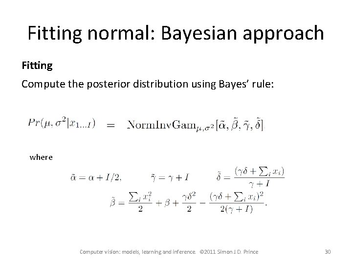
Fitting normal: Bayesian approach Fitting Compute the posterior distribution using Bayes’ rule: where Computer vision: models, learning and inference. © 2011 Simon J. D. Prince 30

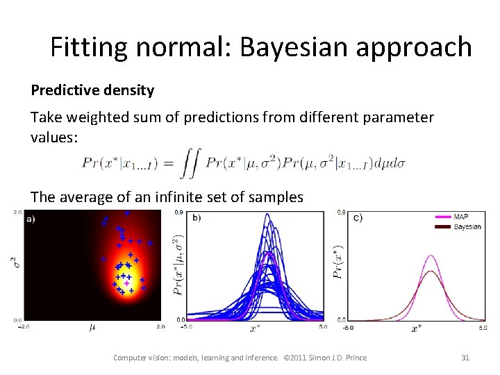
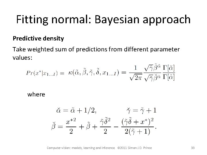
Fitting normal: Bayesian approach Predictive density Take weighted sum of predictions from different parameter values: The average of an infinite set of samples Computer vision: models, learning and inference. © 2011 Simon J. D. Prince 31

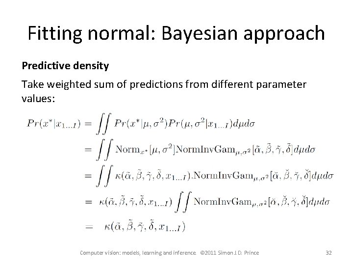
Fitting normal: Bayesian approach Predictive density Take weighted sum of predictions from different parameter values: Computer vision: models, learning and inference. © 2011 Simon J. D. Prince 32

Fitting normal: Bayesian approach Predictive density Take weighted sum of predictions from different parameter values: where Computer vision: models, learning and inference. © 2011 Simon J. D. Prince 33

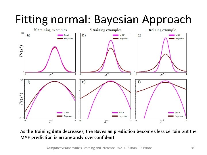
Fitting normal: Bayesian Approach As the training data decreases, the Bayesian prediction becomes less certain but the MAP prediction is erroneously overconfident Computer vision: models, learning and inference. © 2011 Simon J. D. Prince 34

Structure • Fitting probability distributions – Maximum likelihood – Maximum a posteriori – Bayesian approach • Worked example 1: Normal distribution • Worked example 2: Categorical distribution Computer vision: models, learning and inference. © 2011 Simon J. D. Prince 35

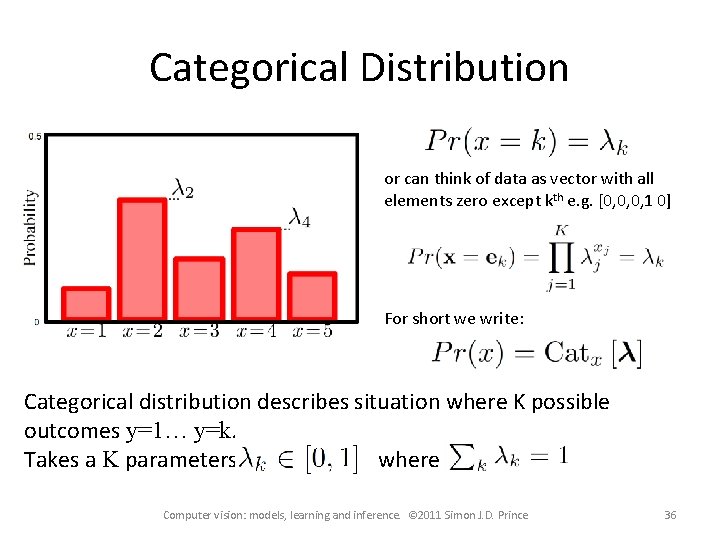
Categorical Distribution or can think of data as vector with all elements zero except kth e. g. [0, 0, 0, 1 0] For short we write: Categorical distribution describes situation where K possible outcomes y=1… y=k. Takes a K parameters where Computer vision: models, learning and inference. © 2011 Simon J. D. Prince 36

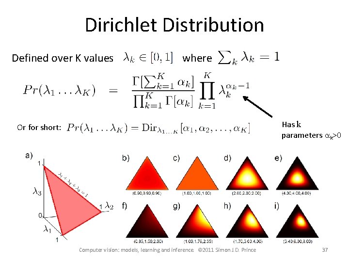
Dirichlet Distribution Defined over K values where Has k parameters ak>0 Or for short: Computer vision: models, learning and inference. © 2011 Simon J. D. Prince 37

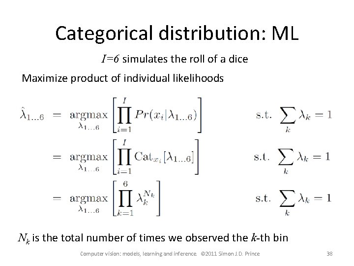
Categorical distribution: ML I=6 simulates the roll of a dice Maximize product of individual likelihoods Nk is the total number of times we observed the k-th bin Computer vision: models, learning and inference. © 2011 Simon J. D. Prince 38

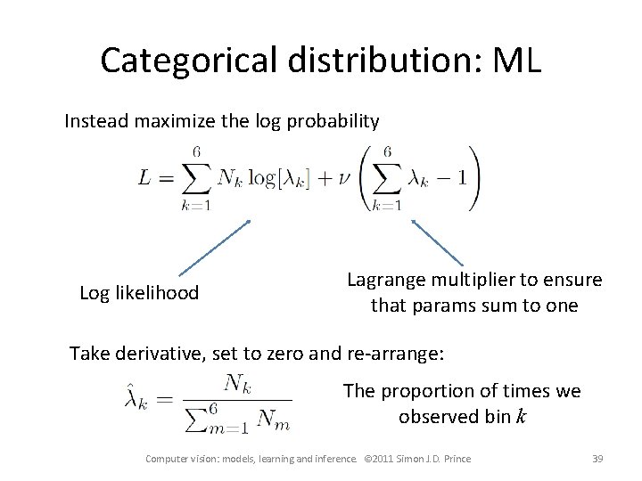
Categorical distribution: ML Instead maximize the log probability Log likelihood Lagrange multiplier to ensure that params sum to one Take derivative, set to zero and re-arrange: The proportion of times we observed bin k Computer vision: models, learning and inference. © 2011 Simon J. D. Prince 39

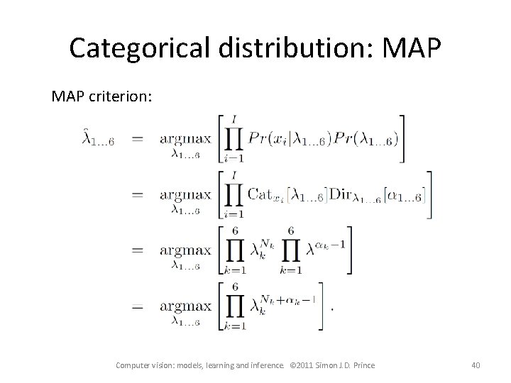
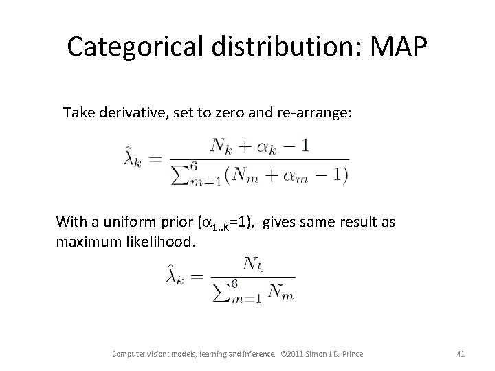
Categorical distribution: MAP criterion: Computer vision: models, learning and inference. © 2011 Simon J. D. Prince 40

Categorical distribution: MAP Take derivative, set to zero and re-arrange: With a uniform prior (a 1. . K=1), gives same result as maximum likelihood. Computer vision: models, learning and inference. © 2011 Simon J. D. Prince 41

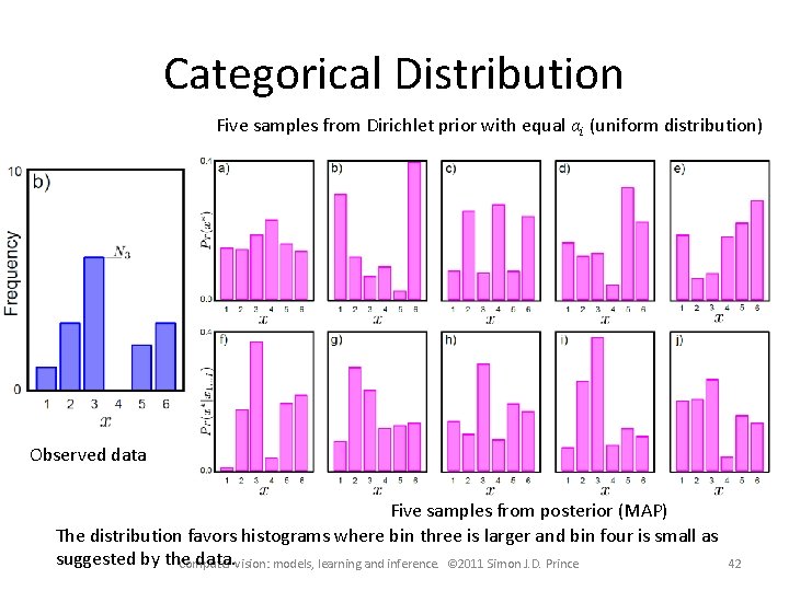
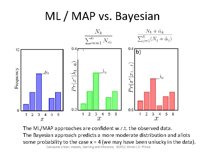
Categorical Distribution Five samples from Dirichlet prior with equal αi (uniform distribution) Observed data Five samples from posterior (MAP) The distribution favors histograms where bin three is larger and bin four is small as suggested by the data. vision: models, learning and inference. © 2011 Simon J. D. Prince Computer 42

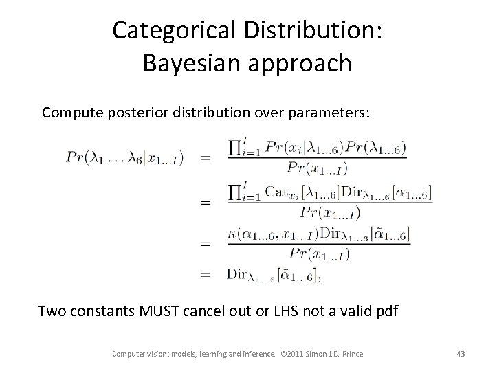
Categorical Distribution: Bayesian approach Compute posterior distribution over parameters: Two constants MUST cancel out or LHS not a valid pdf Computer vision: models, learning and inference. © 2011 Simon J. D. Prince 43

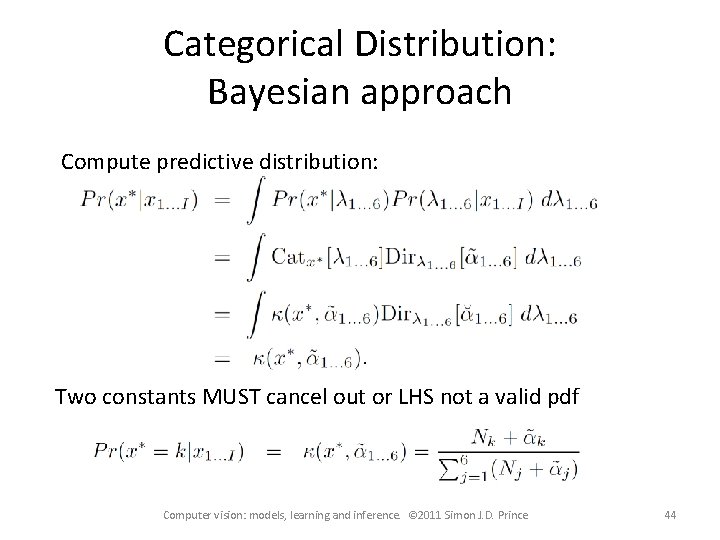
Categorical Distribution: Bayesian approach Compute predictive distribution: Two constants MUST cancel out or LHS not a valid pdf Computer vision: models, learning and inference. © 2011 Simon J. D. Prince 44

ML / MAP vs. Bayesian The ML/MAP approaches are confident w. r. t. the observed data. The Bayesian approach predicts a more moderate distribution and allots some probability to the case x = 4 (we may have been unlucky in the data). Computer vision: models, learning and inference. © 2011 Simon J. D. Prince

Conclusion • Three ways to fit probability distributions • Maximum likelihood • Maximum a posteriori • Bayesian Approach • Two worked example • Normal distribution (ML least squares) • Categorical distribution Computer vision: models, learning and inference. © 2011 Simon J. D. Prince 46