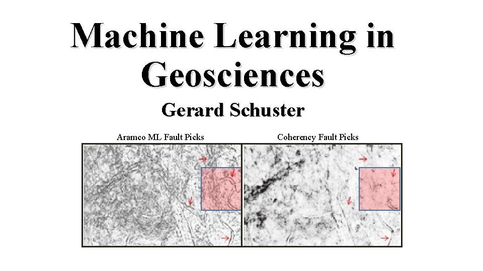
Machine Learning in Geosciences Gerard Schuster Aramco ML

Machine Learning in Geosciences Gerard Schuster Aramco ML Fault Picks Coherency Fault Picks

• • Outline History Three Types of ML & Supervised Learning Neural Network Example: Well Log Neural Network Example: Rock ID Neural Network Example: Migration Neural Network Example: Fault & Lith. ID Summary

Machine Learning Arthur Samuel way back in 1959: “[Machine Learning is the] field of study that gives computers the ability to learn without being explicitly programmed. “ Y = GPA at KAUST Linear regression y=mx+b Geo. Math Phys+Geo x = Background Mary has a physics degree, what is her expected GPA?

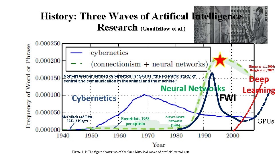
History: Three Waves of Artifical Intelligence Research (Goodfellow et al. ) Hinton et al. , 2006; Bengio et al. , 2007 Norbert Wiener defined cybernetics in 1948 as "the scientific study of control and communication in the animal and the machine. " Neural Networks FWI Cybernetics Mc. Culloch and Pitts 1943 (biology) Rosenblatt, 1958 perceptron 2 -layer Neural Networks (1986) Figure 1. 7: The figure shows two of the three historical waves of artificial neural nets Deep Learning GPUs

• • Outline History Three Types of ML & Supervised Learning Neural Network Example: Well Log Neural Network Example: Rock ID Neural Network Example: Migration Neural Network Example: Fault & Lith. ID Summary

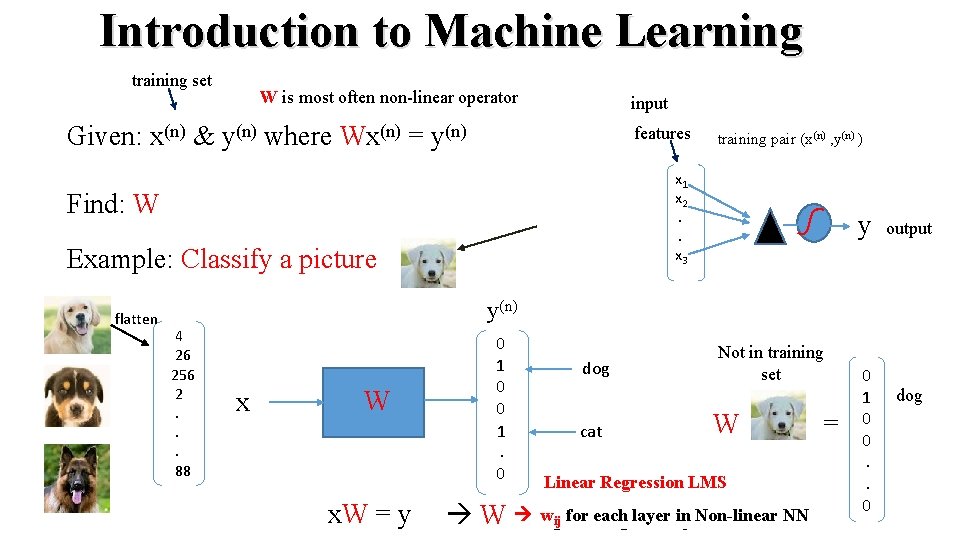
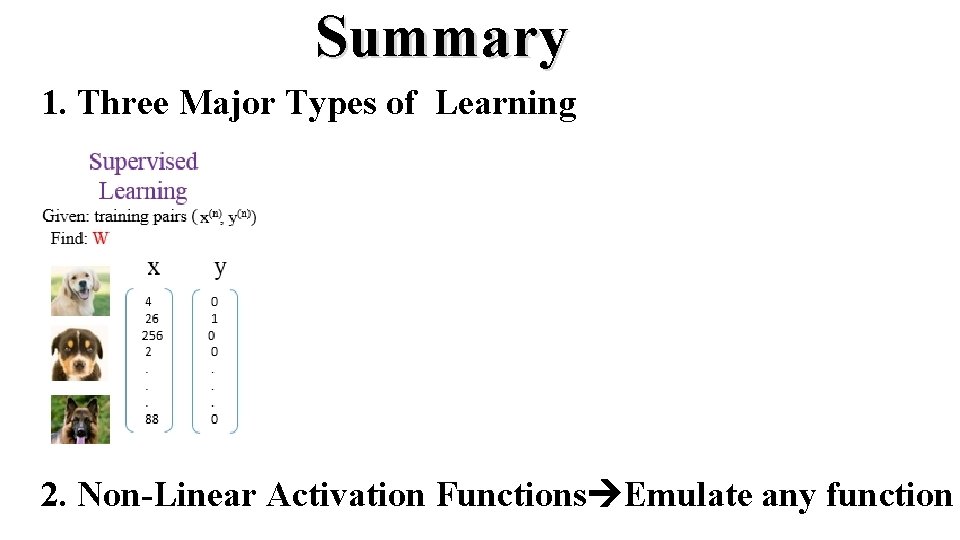
Introduction to Machine Learning training set W is most often non-linear operator input Given: x(n) & y(n) where Wx(n) = y(n) features Find: W then use W to predict y(n+1) from x(n+1) Example: Classify a picture [ x x x ] (1) flatten (2) 4 26 256 2. . . 88 (3) T W x training pair (x(n) , y(n) ) x 1 x 2. . x 3 y output y(n) 0 1 0 0 1. . 0 dog cat Not in training set W = Linear Regression LMS T X]-1 XTy x. W = y W-1 w = [X ij for each layer in Non-linear NN 0 1 0 0. . 0 dog

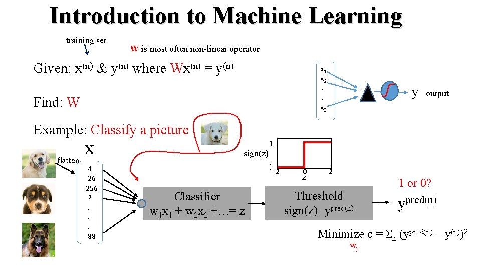
Introduction to Machine Learning training set W is most often non-linear operator Given: x(n) & y(n) where Wx(n) = y(n) Find: W then use W to predict y(n+1) from x(n+1) Example: Classify a picture [ x x ] (1) flatten (2) 4 26 256 2. . . 88 (3) T Classifier y output 1 sign(z) 0 -2 w 1 x 1 + w 2 x 2 +…= z x 1 x 2. . x 3 0 z 2 Threshold sign(z)=ypred(n) 1 or 0? ypred(n) Minimize e = Sn (ypred(n) – y(n))2 wj

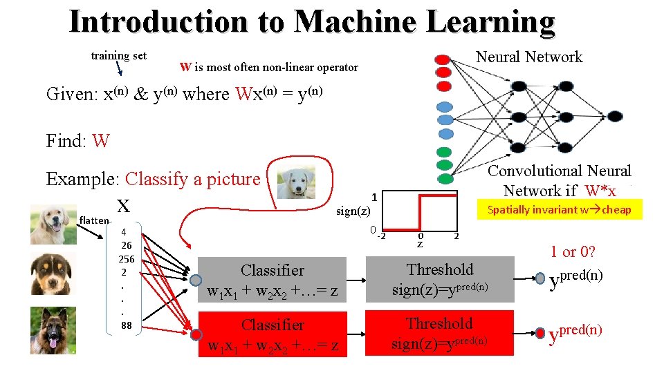
Introduction to Machine Learning training set Neural Network W is most often non-linear operator Given: x(n) & y(n) where Wx(n) = y(n) Find: W then use W to predict y(n+1) from x(n+1) Example: Classify a picture [ x x ] (1) flatten (2) 4 26 256 2. . . 88 (3) T x 1 x 2. . x 3 y Convolutional Neural Network if W*x 1 sign(z) 0 -2 output Spatially invariant w cheap 0 z 2 1 or 0? w 1 x 1 + w 2 x 2 +…= z Threshold sign(z)=ypred(n) Classifier

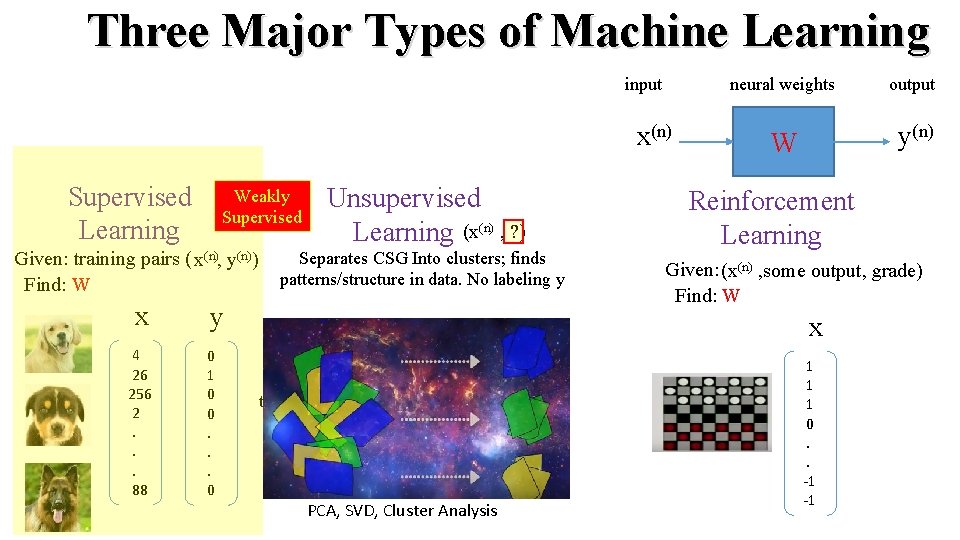
Three Major Types of Machine Learning input neural weights output x(n) Supervised Learning Weakly Supervised Given: training pairs ( x(n), y(n)) Find: W Unsupervised Learning (x(n) , ? ) Separates CSG Into clusters; finds patterns/structure in data. No labeling y x y CSG 4 26 256 2. . . 88 0 1 0 0. . . 0 FK Spectrum Rayleigh FK t w reflection x PCA, SVD, Cluster Analysis kx y(n) W Reinforcement Learning Given: (x(n) , some output, grade) Find: W grade x y 1 1 1 0. . -1 -1 0 1. . . 1 Good if more + than -

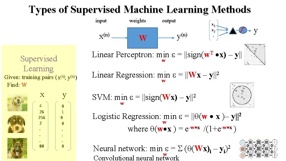
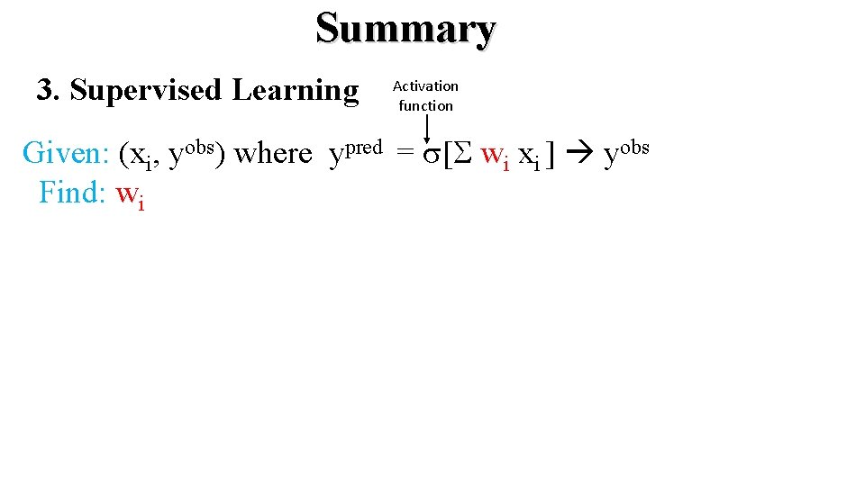
Types of Supervised Machine Learning Methods input weights output x(n) y(n) W x 1 x 2. Linear Perceptron: min e = ||sign(w. T x) – y|| Supervised Learning w Given: training pairs ( x(n), y(n)) Linear Regression: min e = ||Wx – y||2 w Find: W x y SVM: min e = ||sign(Wx) – y||2 4 26 256 2. . . 88 0 1 0 0. . . 0 w Logistic Regression: min e = ||q(w x )– y||2 w where q(w x ) = e-w x /(1+e-w x ) Neural network: min e = S (q(Wx)i – yi)2 w Convolutional neural network y

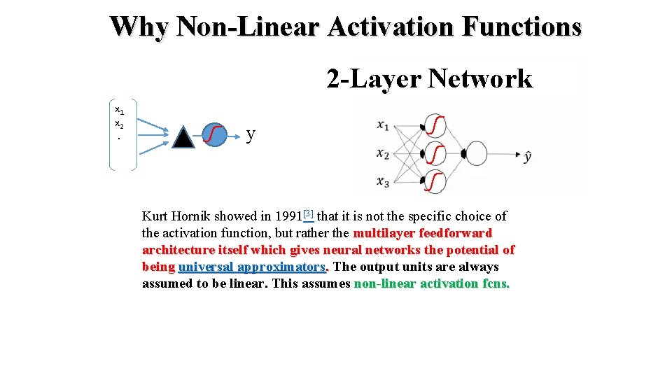
Why Non-Linear Activation Functions 2 -Layer Network x 1 x 2. y Kurt Hornik showed in 1991[3] that it is not the specific choice of the activation function, but rather the multilayer feedforward architecture itself which gives neural networks the potential of being universal approximators. The output units are always . 3 x 1 vector assumed to be linear. This assumes non-linear activation fcns.

• • Outline History Three Types of ML & Supervised Learning Neural Network Example: Well Log Neural Network Example: Rock ID Neural Network Example: Migration Neural Network Example: Fault & Lith. ID Summary

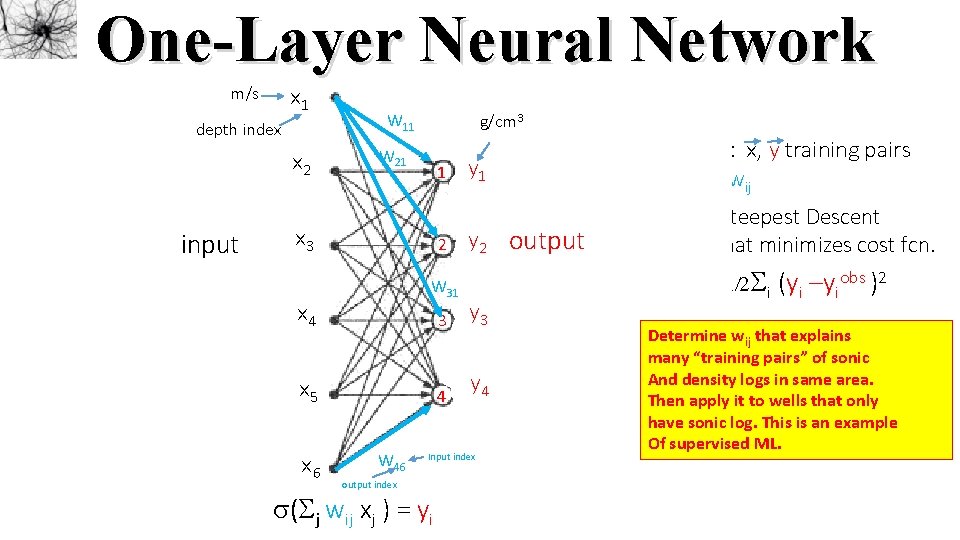
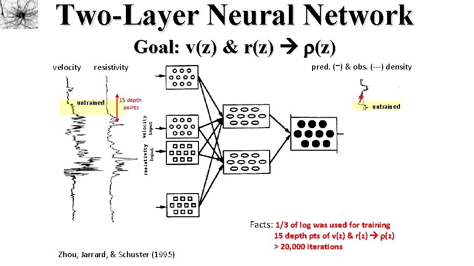
One-Layer Neural Network x V (m/s) x 1 m/s depth index x 2 W 11 y g/cm 3 W 21 1 Given: x, y training pairs Find: wij y 1 Depth 1 input x 3 x 4 Sonic Log 2 y 2 output W 31 2 3 x 5 x 6 4 W 46 output index y 3 y 4 Input index s(Sj wij xj ) = yi 3 Soln: Steepest Descent that minimizes cost fcn. e=1/2 Si (yi –yiobs )2 Determine wij that explains many “training pairs” of sonic And density logs in same area. Density. Then Log apply it to wells that only have sonic log. This is an example Of supervised ML.

Two-Layer Neural Network Goal: v(z) & r(z) velocity - pred. ( ) & obs. (---) density resistivity untrained 15 depth points input * * untrained output Facts: 1/3 of log was used for training Zhou, Jarrard, & Schuster (1995) 15 depth pts of v(z) & r(z) > 20, 000 iterations

• • Outline History Three Types of ML & Supervised Learning Neural Network Example: Well Log Neural Network Example: Rock Classification Neural Network Example: Migration Neural Network Example: Fault & Lith. ID Summary

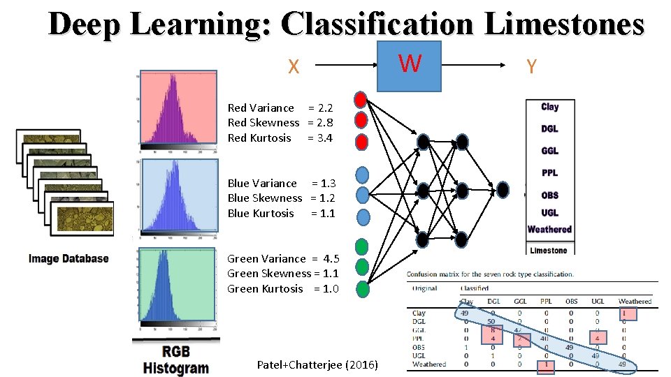
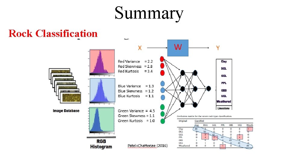
Deep Learning: Classification Limestones X Red Variance = 2. 2 Red Skewness = 2. 8 Red Kurtosis = 3. 4 Blue Variance = 1. 3 Blue Skewness = 1. 2 Blue Kurtosis = 1. 1 Green Variance = 4. 5 Green Skewness = 1. 1 Green Kurtosis = 1. 0 Patel+Chatterjee (2016) W Y

• • Outline History Three Types of ML & Supervised Learning Neural Network Example: Well Log Neural Network Example: Rock Classification Neural Network Example: Migration Neural Network Example: Fault & Lith. ID Summary

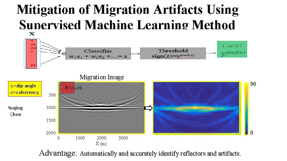
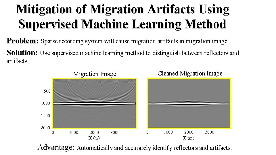
Mitigation of Migration Artifacts Using Supervised Machine Learning Method Problem: Sparse recording system will cause migration artifacts in migration image. Solution: Use supervised machine learning method to distinguish between reflectors and artifacts. Migration Image a=dip angle s=coherency Yuqing Chen Xx=(a, s) 500 Interpreted Migration Image 0 Y= 1 90 1000 1500 2000 0 1000 2000 3000 X (m) Advantage: Automatically and accurately identify reflectors and artifacts. 0

• • Outline History Three Types of ML & Supervised Learning Neural Network Example: Well Log Neural Network Example: Rock Classification Neural Network Example: Migration Neural Network Example: Fault & Lith. ID Summary

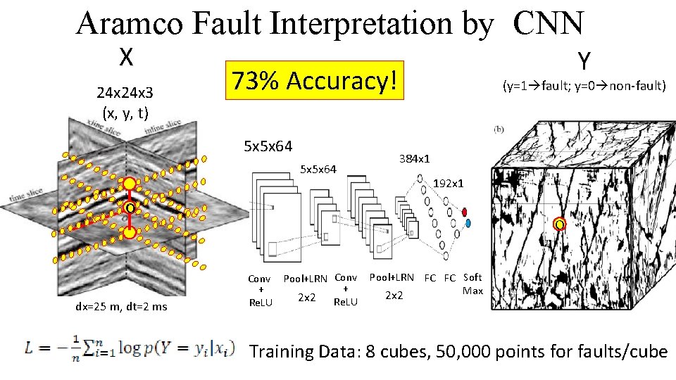
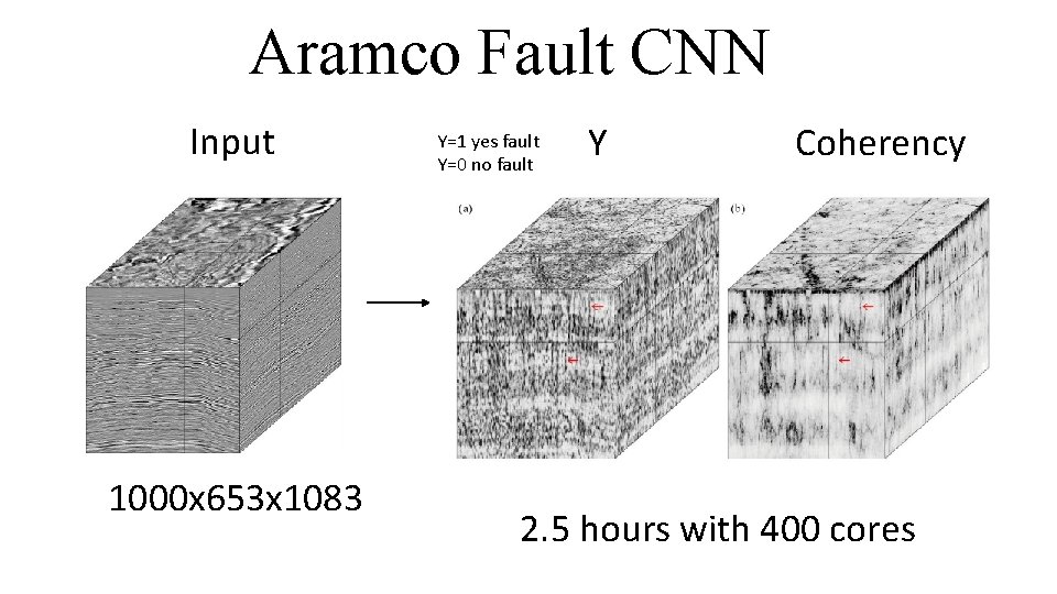
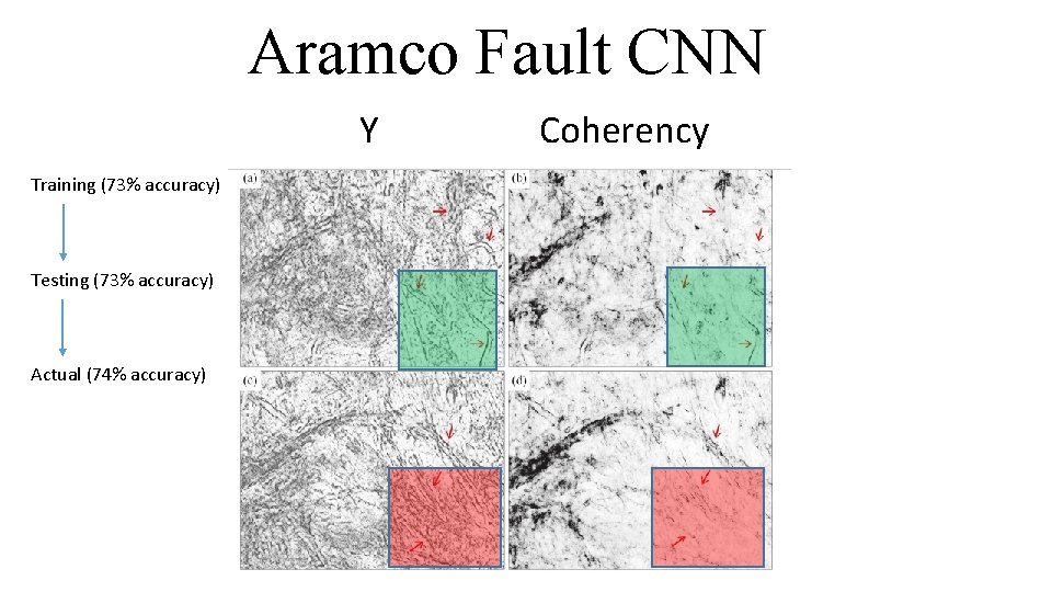
Aramco Fault Interpretation by CNN X 24 x 3 (x, y, t) Y 73% Accuracy! 5 x 5 x 64 (y=1 fault; y=0 non-fault) 384 x 1 192 x 1 o dx=25 m, dt=2 ms o Conv Pool+LRN Conv + + 2 x 2 Re. LU Pool+LRN FC FC Soft Max 2 x 2 Training Data: 8 cubes, 50, 000 points for faults/cube

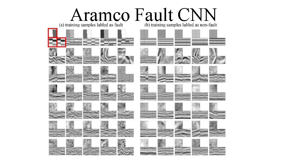
Aramco Fault CNN

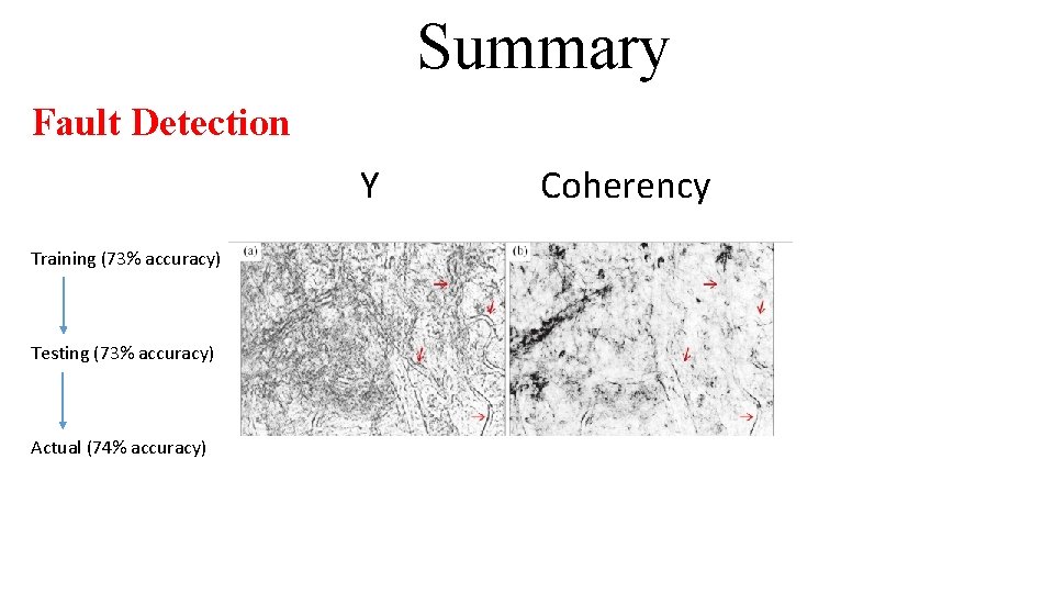
Aramco Fault CNN Input 1000 x 653 x 1083 Y=1 yes fault Y=0 no fault Y Coherency 2. 5 hours with 400 cores

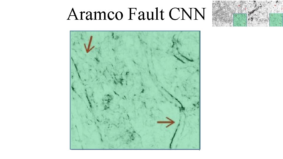
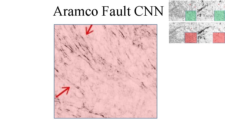
Aramco Fault CNN Y Training (73% accuracy) Testing (73% accuracy) Actual (74% accuracy) Coherency

Aramco Fault CNN

Aramco Fault CNN

• • Outline History Three Types of ML & Supervised Learning Neural Network Example: Well Log Neural Network Example: Rock Classification Neural Network Example: Migration Neural Network Example: Fault & Salt ID Summary

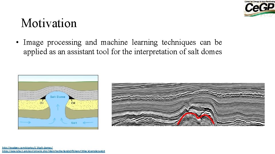
Motivation • Image processing and machine learning techniques can be applied as an assistant tool for the interpretation of salt domes http: //geology. com/stories/13/salt-domes/ https: //opendtect. org/osr/pmwiki. php/Main/Netherlands. Offshore. F 3 Block. Complete 4 GB

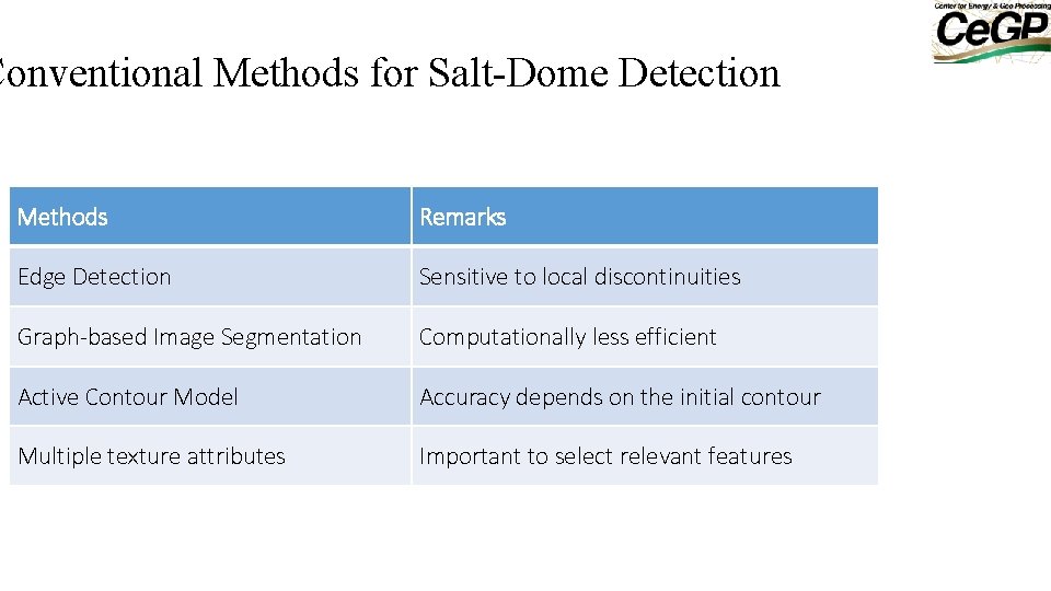
Conventional Methods for Salt-Dome Detection Methods Remarks Edge Detection Sensitive to local discontinuities Graph-based Image Segmentation Computationally less efficient Active Contour Model Accuracy depends on the initial contour Multiple texture attributes Important to select relevant features

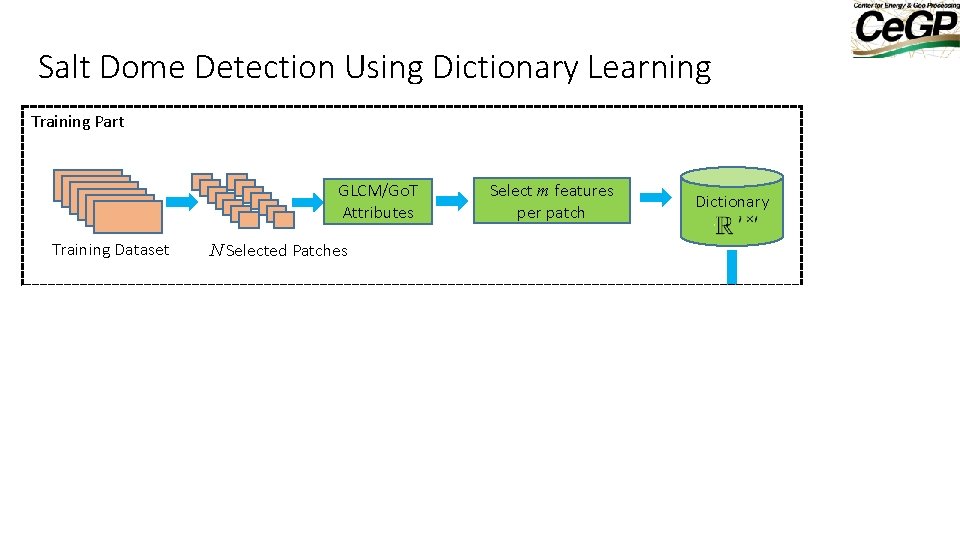
Salt Dome Detection Using Dictionary Learning Training Part GLCM/Go. T Attributes Training Dataset Select m features per patch N Selected Patches Classify each patch as 1. Salt Boundary 2. Non Salt Boundary Post-processing Solve GLCM/Go. T Attributes Seismic Image Detection Part Dictionary Non-overlapped Patches minimization

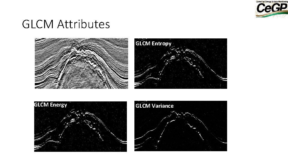
GLCM Attributes GLCM Entropy GLCM Energy GLCM Variance

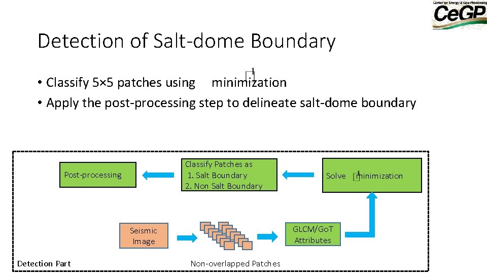
Detection of Salt-dome Boundary • Classify 5× 5 patches using minimization • Apply the post-processing step to delineate salt-dome boundary Classify Patches as 1. Salt Boundary 2. Non Salt Boundary Post-processing GLCM/Go. T Attributes Seismic Image Detection Part Solve Non-overlapped Patches minimization

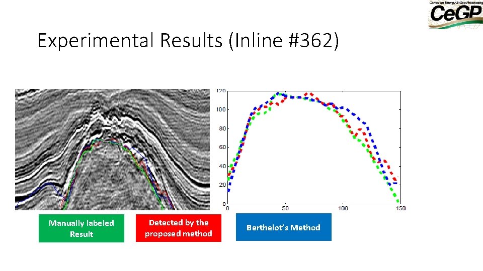
Experimental Results (Inline #362) Manually labeled Result Detected by the proposed method Berthelot’s Method

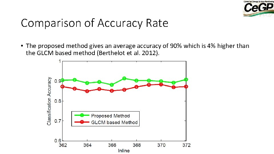
Comparison of Accuracy Rate • The proposed method gives an average accuracy of 90% which is 4% higher than the GLCM based method (Berthelot et al. 2012).

• • Outline History Three Types of ML & Supervised Learning Neural Network Example: Well Log Neural Network Example: Rock Classification Neural Network Example: Migration Neural Network Example: Fault & Lith. ID Summary

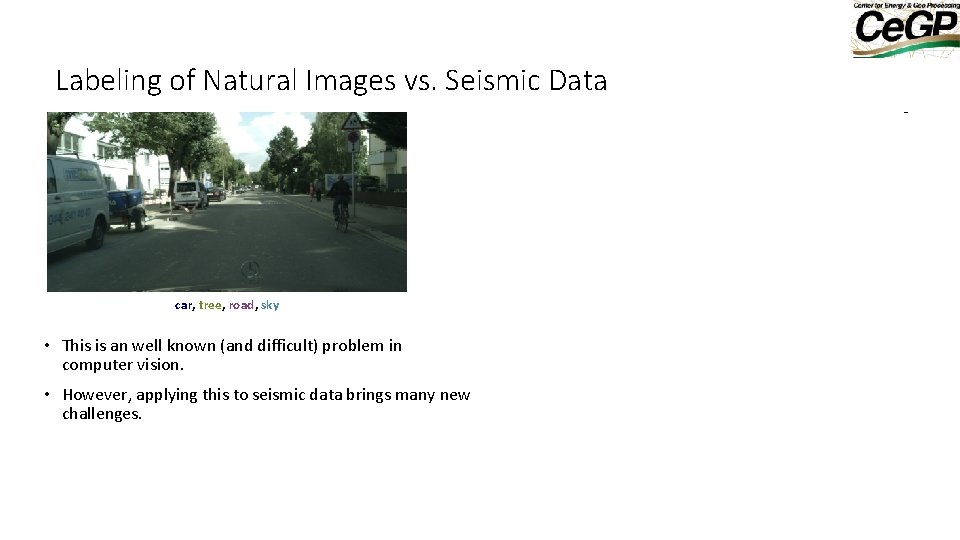
Labeling of Natural Images vs. Seismic Data tree sky car road car, tree, road, sky • This is an well known (and difficult) problem in computer vision. • However, applying this to seismic data brings many new challenges. 1. Seismic data doesn’t have color information. 2. Subsurface structures are characterized by texture, and lack the clearly defined boundaries between objects in the natural world 3. Severe lack of labeled seismic data

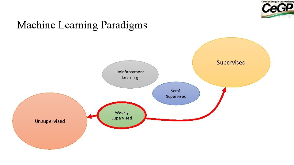
Machine Learning Paradigms Supervised Reinforcement Learning Semi. Supervised Unsupervised Weakly Supervised

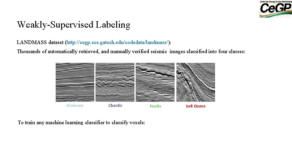
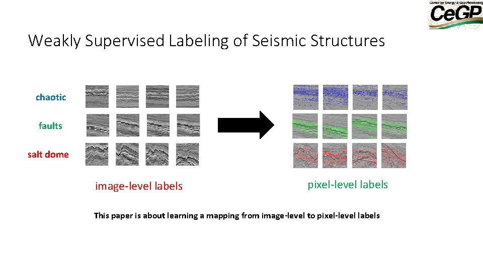
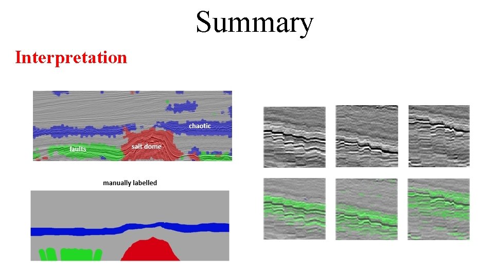
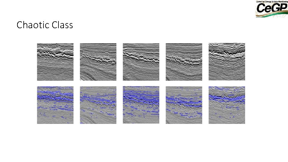
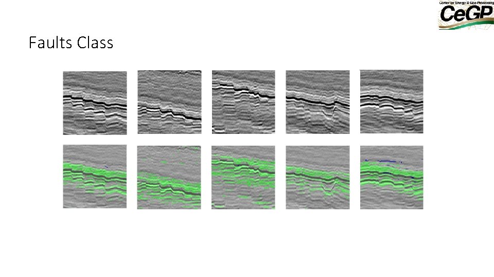
Weakly-Supervised Labeling LANDMASS dataset (http: //cegp. ece. gatech. edu/codedata/landmass/): Thousands of automatically retrieved, and manually verified seismic images classified into four classes: Horizons Chaotic Faults To train any machine learning classifier to classify voxels: - ideally you would have labeled pixels supervised learning - If we only have image-level labels weakly-supervised learning Salt Dome

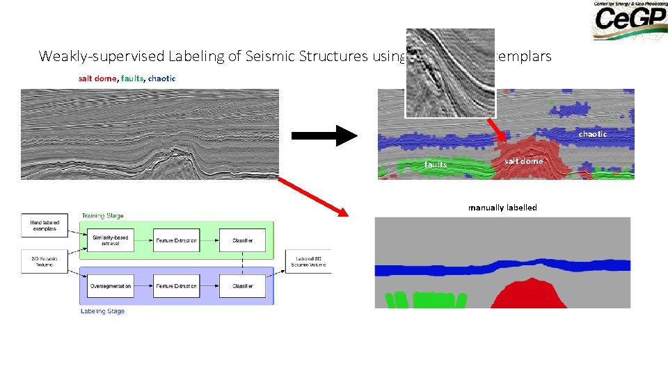
Weakly-supervised Labeling of Seismic Structures using Reference Exemplars salt dome, faults, chaotic faults salt dome manually labelled

Weakly Supervised Labeling of Seismic Structures chaotic faults salt dome image-level labels pixel-level labels This paper is about learning a mapping from image-level to pixel-level labels

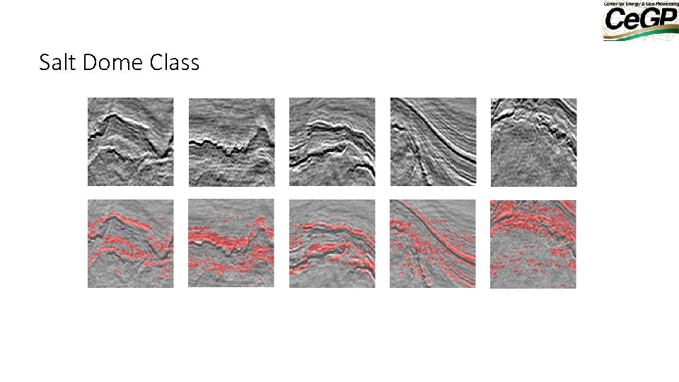
Salt Dome Class

Outline • • • History+Example Course Three Types of ML & Supervised Learning Neural Network Example: Well Log Neural Network Example: Lithology Ident. Summary

Summary 1. Three Major Types of Learning 2. Non-Linear Activation Functions Emulate any function

Summary 3. Supervised Learning Activation function Given: (xi, yobs) where ypred = s[S wi xi ] yobs Find: wi CNN linear regression logistic regression ypred = (S wi xi ) ypred = q(S wi xi ) x 1 x 2. . x 3 Swi ypred x 1 x 2. . x 3 1/(1+e-z) Swi ypred 1/(1+e-z)

Issues in Machine Learning 1. 2. 3. 4. 5. 6. 7. Convergence Rate? Local Minima? Design of Neural Network Architecture? Best Input Features? Physics+ML Optimal Combination? How Much Training Needed? Sanity Checks of Predictions?

Summary Fault Detection Y Coherency Training (73% accuracy) Testing (73% accuracy) Actual (74% accuracy) • 0. 2% of original data used for training • 2. 5 hours prediction 400 cores • 3 D convolution too expensive for now

Summary Interpretation

Summary Rock Classification

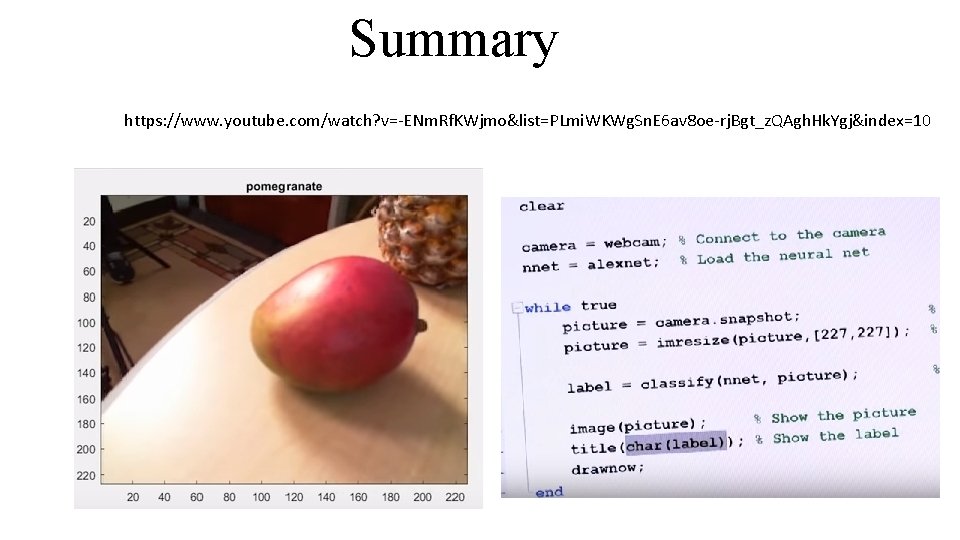
Summary https: //www. youtube. com/watch? v=-ENm. Rf. KWjmo&list=PLmi. WKWg. Sn. E 6 av 8 oe-rj. Bgt_z. QAgh. Hk. Ygj&index=10

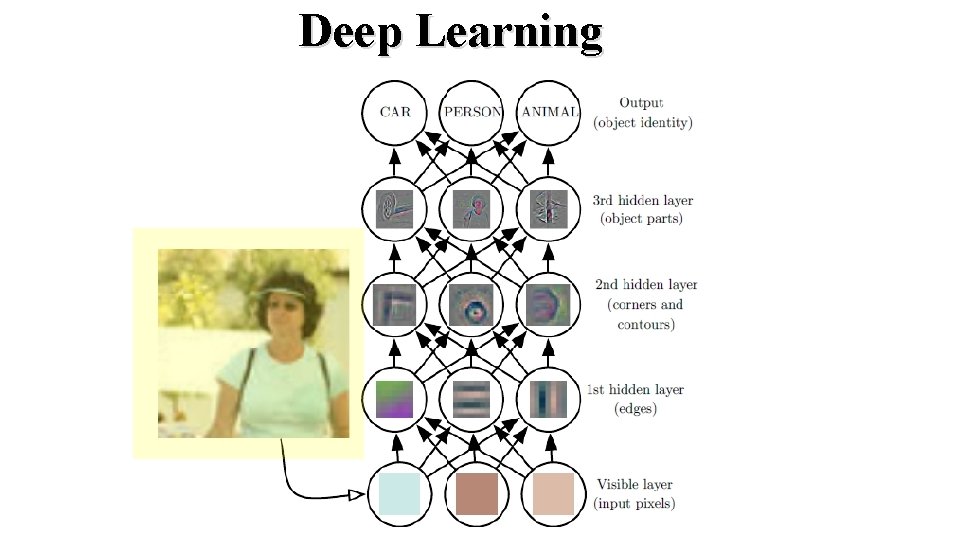
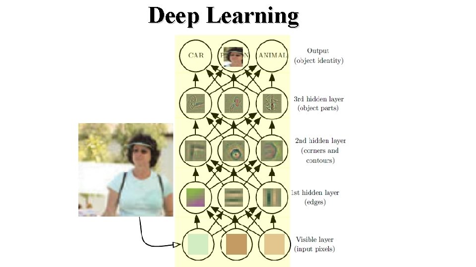
Deep Learning

Deep Learning

Deep Learning: Classification Limestones X Red Variance = 2. 2 Red Skewness = 2. 8 Red Kurtosis = 3. 4 Blue Variance = 1. 3 Blue Skewness = 1. 2 Blue Kurtosis = 1. 1 Green Variance = 4. 5 Green Skewness = 1. 1 Green Kurtosis = 1. 0 Patel+Chatterjee (2016) W Y

Outline • • History+Example Course Three Types of ML & Supervised Learning Neural Network Example: Well Log Neural Network Example: Migration Deep Learning Summary

Summary 1. Three Major Types of Learning 2. Non-Linear Activation Functions Emulate any function

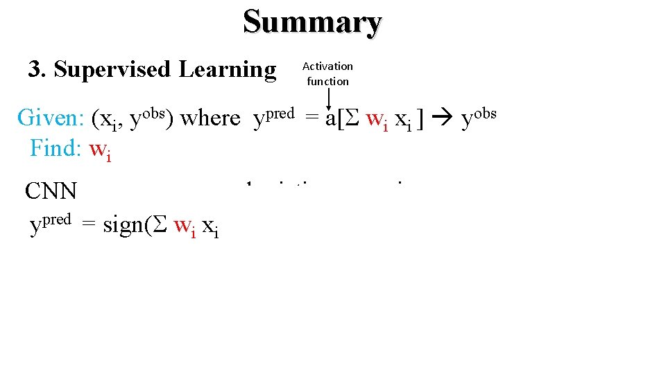
Summary 3. Supervised Learning Activation function Given: (xi, yobs) where ypred = a[S wi xi ] yobs Find: wi CNN logistic regression ypred = sign(S wi xi ) ypred = q(S wi xi ) x 1 x 2. . x 3 Swi ypred x 1 x 2. . x 3 1/(1+e-z) Swi ypred 1/(1+e-z)

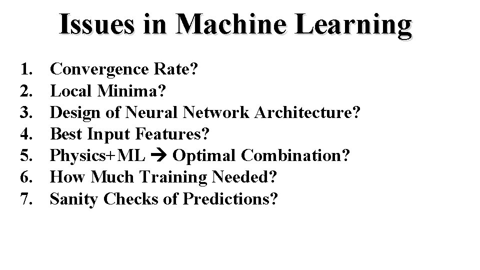
Issues in Machine Learning 1. 2. 3. 4. 5. 6. 7. Convergence Rate? Local Minima? Design of Neural Network Architecture? Best Input Features? Physics+ML Optimal Combination? How Much Training Needed? Sanity Checks of Predictions?

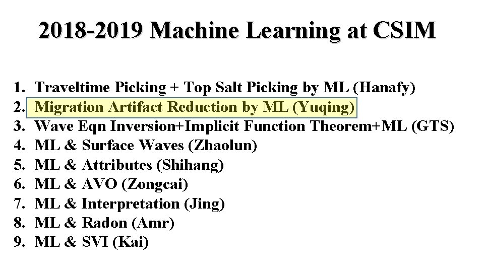
2018 -2019 Machine Learning at CSIM 1. 2. 3. 4. 5. 6. 7. 8. 9. Traveltime Picking + Top Salt Picking by ML (Hanafy) Migration Artifact Reduction by ML (Yuqing) Wave Eqn Inversion+Implicit Function Theorem+ML (GTS) ML & Surface Waves (Zhaolun) ML & Attributes (Shihang) ML & AVO (Zongcai) ML & Interpretation (Jing) ML & Radon (Amr) ML & SVI (Kai)

Mitigation of Migration Artifacts Using Supervised Machine Learning Method Problem: Sparse recording system will cause migration artifacts in migration image. Solution: Use supervised machine learning method to distinguish between reflectors and artifacts. Migration Image Cleaned Migration Image 500 1000 1500 2000 0 1000 2000 3000 X (m) Advantage: Automatically and accurately identify reflectors and artifacts.

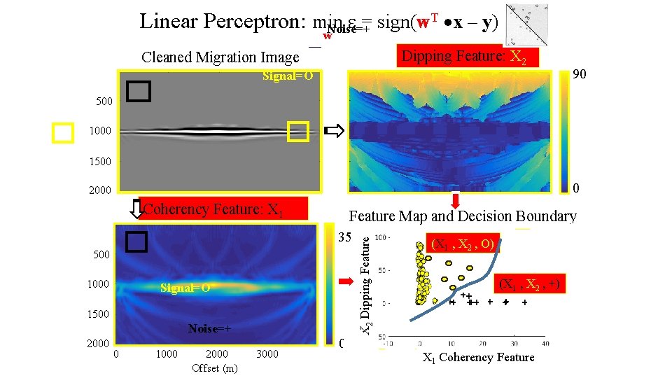
T x – y) w Linear Perceptron: min e = sign(w w. Noise=+ Dipping Feature: X 2 Noisy Migration Image Cleaned Migration Image Signal=O 90 500 1000 1500 0 2000 Coherency Feature: X 1 35 500 1000 Signal=O 1500 Noise=+ 2000 0 1000 2000 3000 Offset (m) 0 X 2 Dipping Feature Map and Decision Boundary (X 1 , X 2 , O) (X 1 , X 2 , +) X 1 Coherency Feature

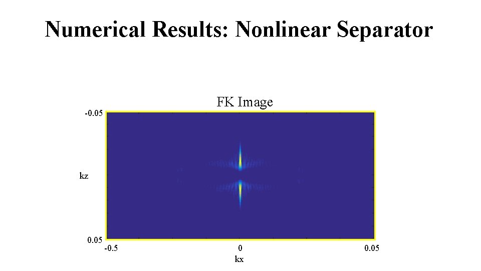
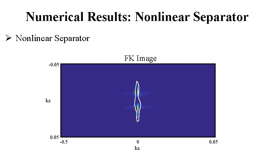
Numerical Results: Nonlinear Separator Ø Nonlinear Separator -0. 05 FK Image kz 0. 05 -0. 5 0. 05 kx

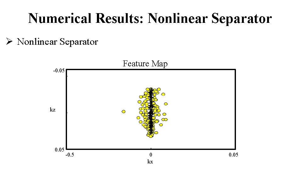
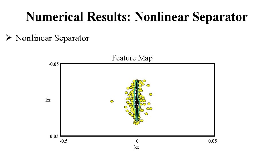
Numerical Results: Nonlinear Separator Ø Nonlinear Separator -0. 05 Feature Map kz 0. 05 -0. 5 0. 05 kx

Numerical Results: Nonlinear Separator Ø Nonlinear Separator -0. 05 Feature Map kz 0. 05 -0. 5 0. 05 kx

Chaotic Class

Faults Class

Numerical Results: Nonlinear Separator Ø Nonlinear Separator -0. 05 FK Image kz 0. 05 -0. 5 0. 05 kx

Other Stuff

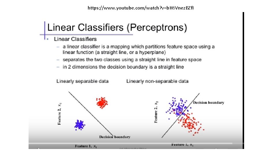
https: //www. youtube. com/watch? v=b. H 6 Vnez. BZf. I

https: //www. youtube. com/watch? v=b. H 6 Vnez. BZf. I

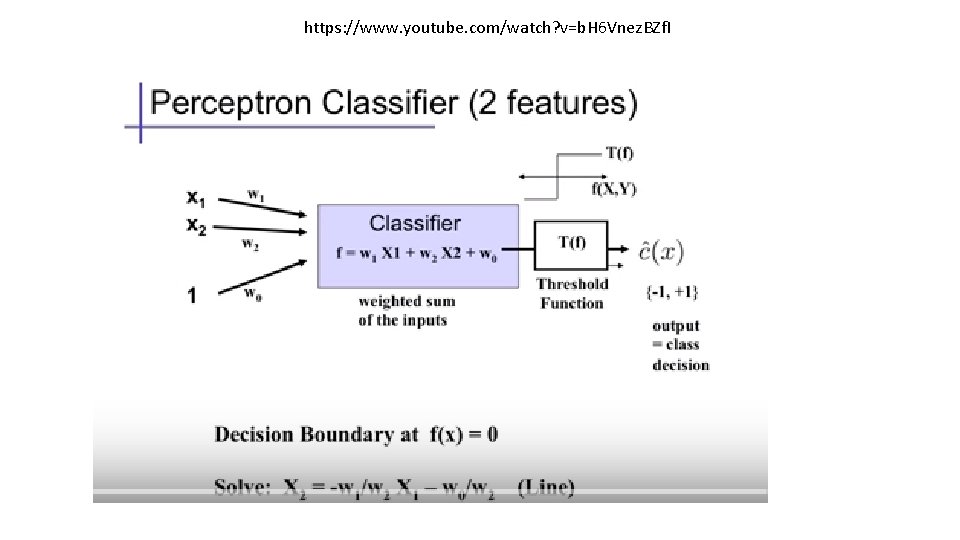
https: //www. youtube. com/watch? v=b. H 6 Vnez. BZf. I

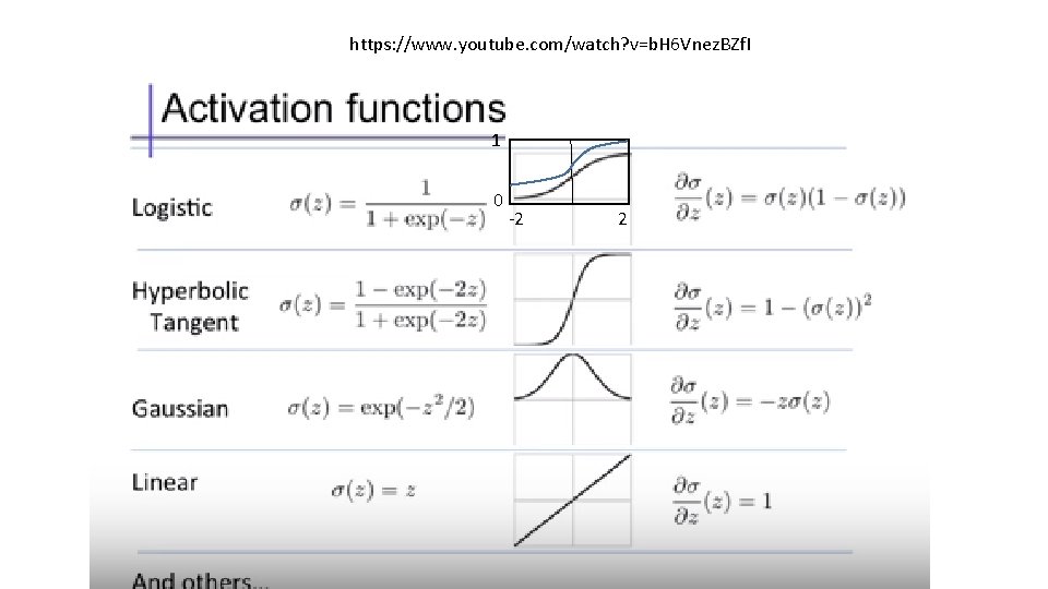
https: //www. youtube. com/watch? v=b. H 6 Vnez. BZf. I 1 0 -2 2

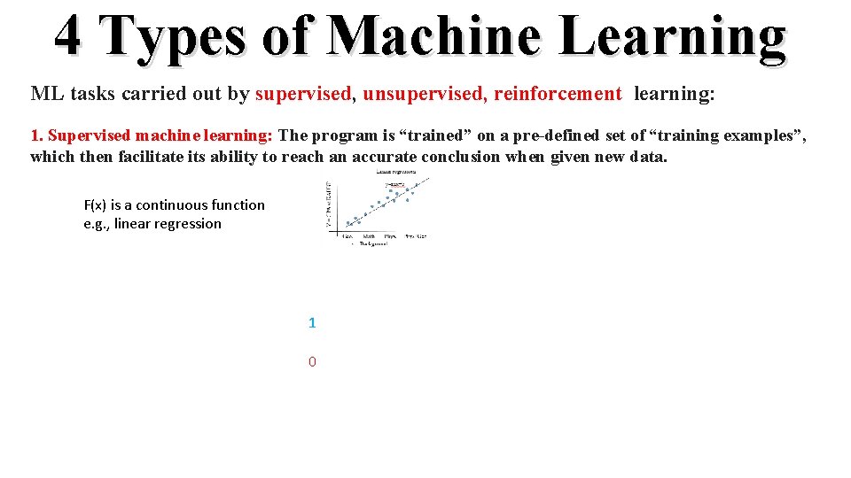
4 Types of Machine Learning ML tasks carried out by supervised, unsupervised, reinforcement learning: 1. Supervised machine learning: The program is “trained” on a pre-defined set of “training examples”, which then facilitate its ability to reach an accurate conclusion when given new data. F(x) is a continuous function e. g. , linear regression 1 F(x) is a discrete function 0 Non-malig. malig Discrete supervised machine learning via Classification: Tumor size

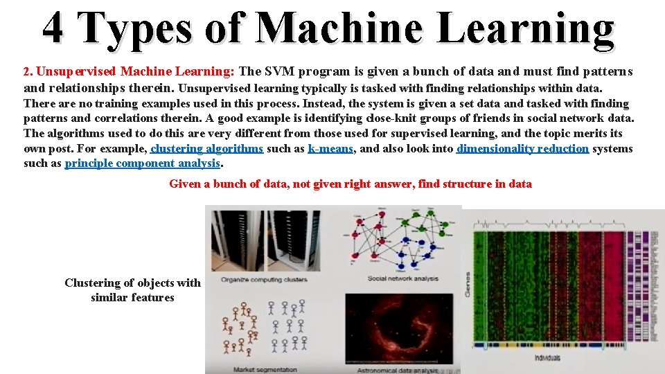
4 Types of Machine Learning 2. Unsupervised Machine Learning: The SVM program is given a bunch of data and must find patterns and relationships therein. Unsupervised learning typically is tasked with finding relationships within data. There are no training examples used in this process. Instead, the system is given a set data and tasked with finding patterns and correlations therein. A good example is identifying close-knit groups of friends in social network data. The algorithms used to do this are very different from those used for supervised learning, and the topic merits own post. For example, clustering algorithms such as k-means, and also look into dimensionality reduction systems such as principle component analysis. Given a bunch of data, not given right answer, find structure in data 1 Clustering of objects with similar features 0 Non-malig. ? Malig? 3 D walkthroughs Stanford campus Tumor size

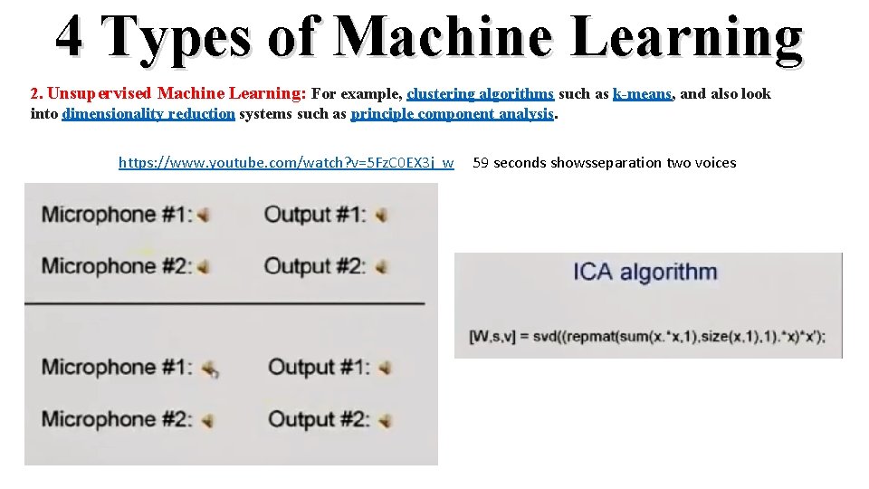
4 Types of Machine Learning 2. Unsupervised Machine Learning: For example, clustering algorithms such as k-means, and also look into dimensionality reduction systems such as principle component analysis. https: //www. youtube. com/watch? v=5 Fz. C 0 EX 3 j_w 59 seconds showsseparation two voices

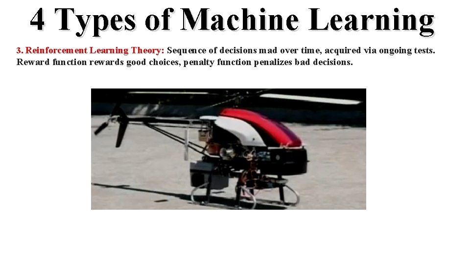
4 Types of Machine Learning 3. Reinforcement Learning Theory: Sequence of decisions mad over time, acquired via ongoing tests. Reward function rewards good choices, penalty function penalizes bad decisions.

4 Types of Machine Learning 4. Learning Theory: When can you expect learning algorithms to work. Theorems can guarantee 99% Accuracy of prediction. Validity of approximations. How many training sets needed to learn properly.

Dip angle w. T x) – y] Linear Perceptron: min e = [sign(w w Dipping Feature: X 2 Noisy Migration Image 90 500 1000 1500 Input: (x 1 , x 2) =(dip angle, coherency value X , X 2) Output: signal(O) or Noise(+) 0 2000 Coherency Feature: X 1 35 Yuqing Chen 500 1000 1500 2000 0 1000 2000 3000 Offset (m) 0 X 2 Dipping Feature Map and Decision Boundary (X 1 , X 2 , +) (X 1 , X 2 , O) X X 11 Coherency Feature

Summary