Computer vision models learning and inference Chapter 13

Computer vision: models, learning and inference Chapter 13 Image preprocessing and feature extraction Please send errata to s. prince@cs. ucl. ac. uk

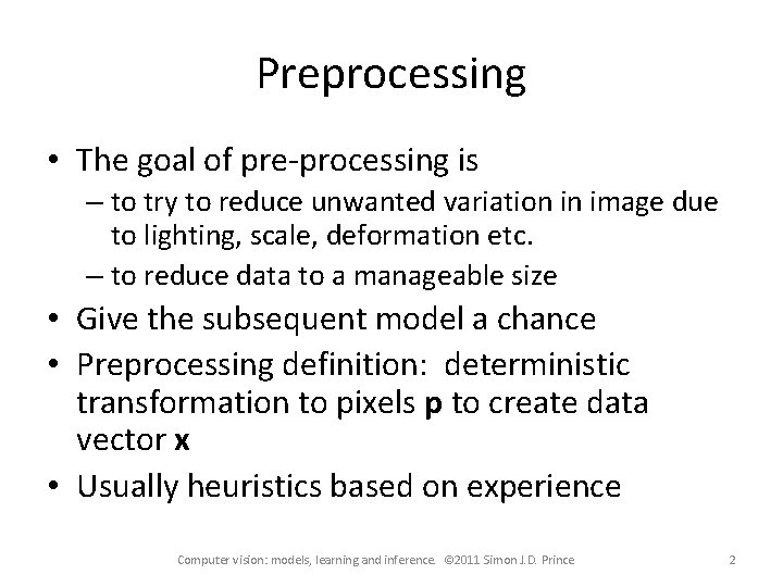
Preprocessing • The goal of pre-processing is – to try to reduce unwanted variation in image due to lighting, scale, deformation etc. – to reduce data to a manageable size • Give the subsequent model a chance • Preprocessing definition: deterministic transformation to pixels p to create data vector x • Usually heuristics based on experience Computer vision: models, learning and inference. © 2011 Simon J. D. Prince 2

Structure • • Per-pixel transformations Edges, corners, and interest points Descriptors Dimensionality reduction Computer vision: models, learning and inference. © 2011 Simon J. D. Prince 3

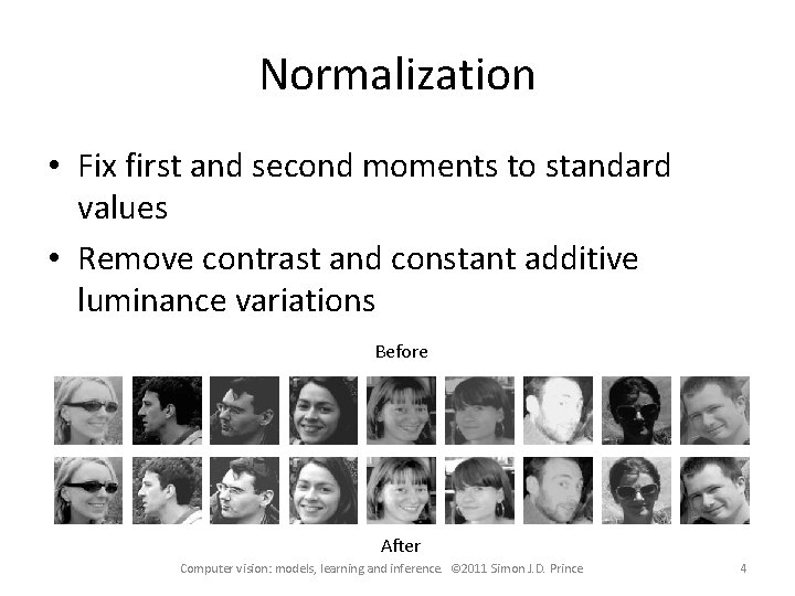
Normalization • Fix first and second moments to standard values • Remove contrast and constant additive luminance variations Before After Computer vision: models, learning and inference. © 2011 Simon J. D. Prince 4

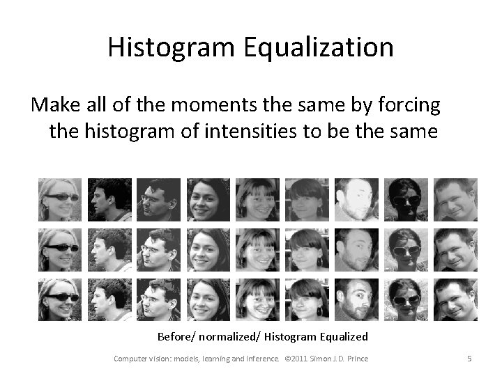
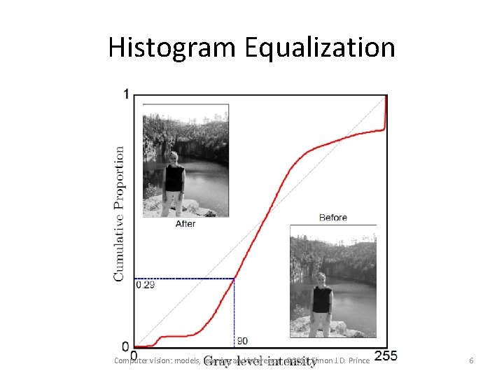
Histogram Equalization Make all of the moments the same by forcing the histogram of intensities to be the same Before/ normalized/ Histogram Equalized Computer vision: models, learning and inference. © 2011 Simon J. D. Prince 5

Histogram Equalization Computer vision: models, learning and inference. © 2011 Simon J. D. Prince 6

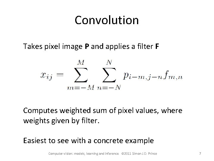
Convolution Takes pixel image P and applies a filter F Computes weighted sum of pixel values, where weights given by filter. Easiest to see with a concrete example Computer vision: models, learning and inference. © 2011 Simon J. D. Prince 7

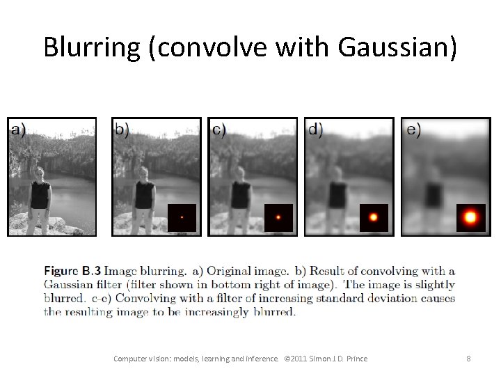
Blurring (convolve with Gaussian) Computer vision: models, learning and inference. © 2011 Simon J. D. Prince 8

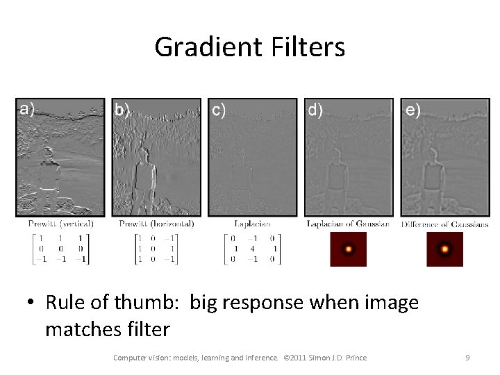
Gradient Filters • Rule of thumb: big response when image matches filter Computer vision: models, learning and inference. © 2011 Simon J. D. Prince 9

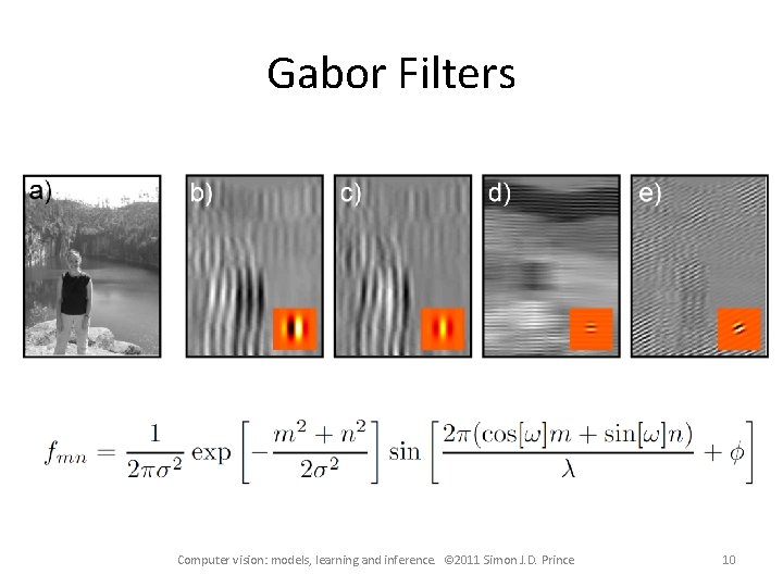
Gabor Filters Computer vision: models, learning and inference. © 2011 Simon J. D. Prince 10

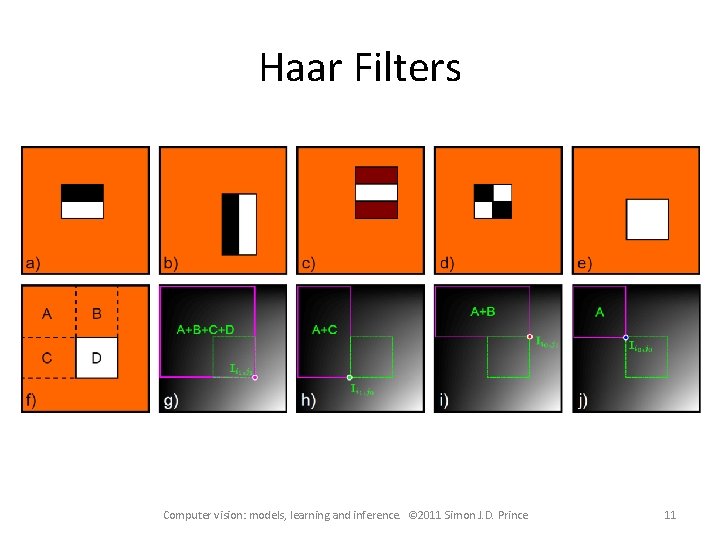
Haar Filters Computer vision: models, learning and inference. © 2011 Simon J. D. Prince 11

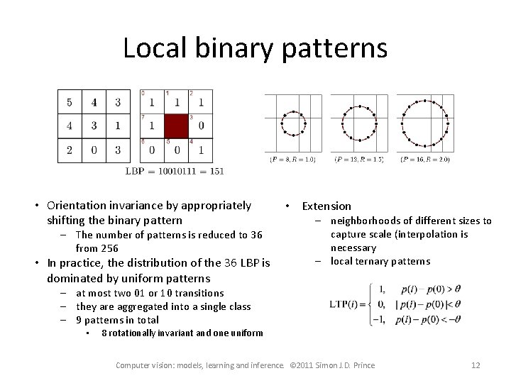
Local binary patterns • Orientation invariance by appropriately shifting the binary pattern – The number of patterns is reduced to 36 from 256 • In practice, the distribution of the 36 LBP is dominated by uniform patterns • Extension – neighborhoods of different sizes to capture scale (interpolation is necessary – local ternary patterns – at most two 01 or 10 transitions – they are aggregated into a single class – 9 patterns in total • 8 rotationally invariant and one uniform Computer vision: models, learning and inference. © 2011 Simon J. D. Prince 12

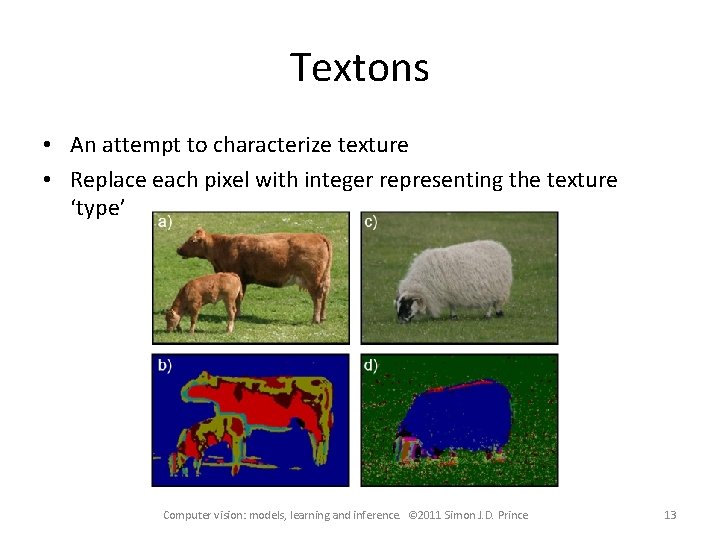
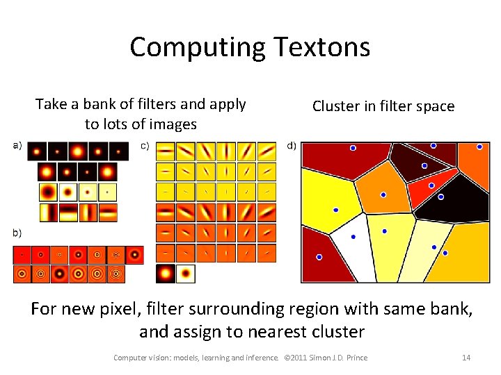
Textons • An attempt to characterize texture • Replace each pixel with integer representing the texture ‘type’ Computer vision: models, learning and inference. © 2011 Simon J. D. Prince 13

Computing Textons Take a bank of filters and apply to lots of images Cluster in filter space For new pixel, filter surrounding region with same bank, and assign to nearest cluster Computer vision: models, learning and inference. © 2011 Simon J. D. Prince 14

Structure • • Per-pixel transformations Edges, corners, and interest points Descriptors Dimensionality reduction Computer vision: models, learning and inference. © 2011 Simon J. D. Prince 15

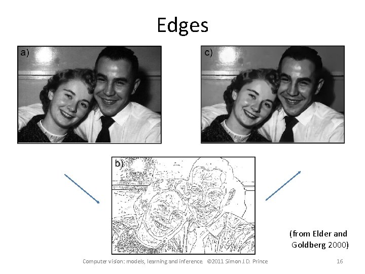
Edges (from Elder and Goldberg 2000) Computer vision: models, learning and inference. © 2011 Simon J. D. Prince 16

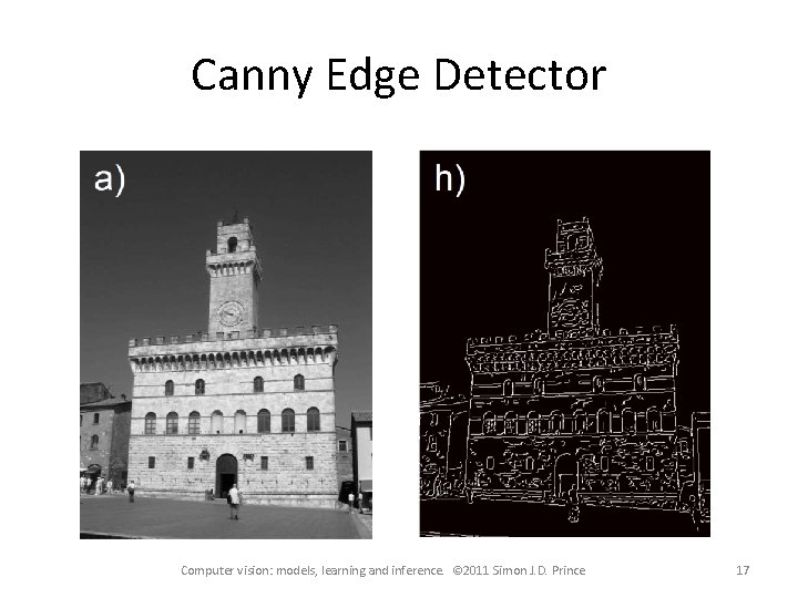
Canny Edge Detector Computer vision: models, learning and inference. © 2011 Simon J. D. Prince 17

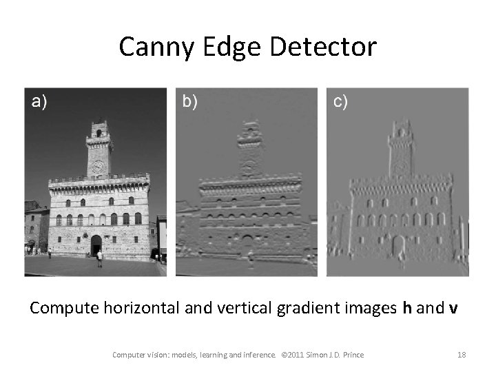
Canny Edge Detector Compute horizontal and vertical gradient images h and v Computer vision: models, learning and inference. © 2011 Simon J. D. Prince 18

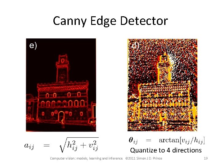
Canny Edge Detector Quantize to 4 directions Computer vision: models, learning and inference. © 2011 Simon J. D. Prince 19

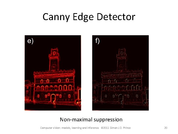
Canny Edge Detector Non-maximal suppression Computer vision: models, learning and inference. © 2011 Simon J. D. Prince 20

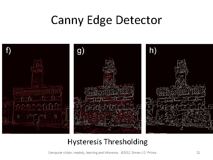
Canny Edge Detector Hysteresis Thresholding Computer vision: models, learning and inference. © 2011 Simon J. D. Prince 21

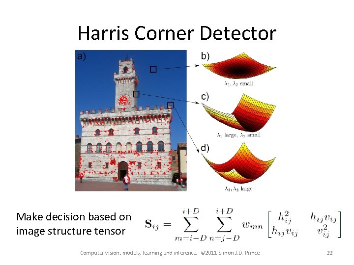
Harris Corner Detector Make decision based on image structure tensor Computer vision: models, learning and inference. © 2011 Simon J. D. Prince 22

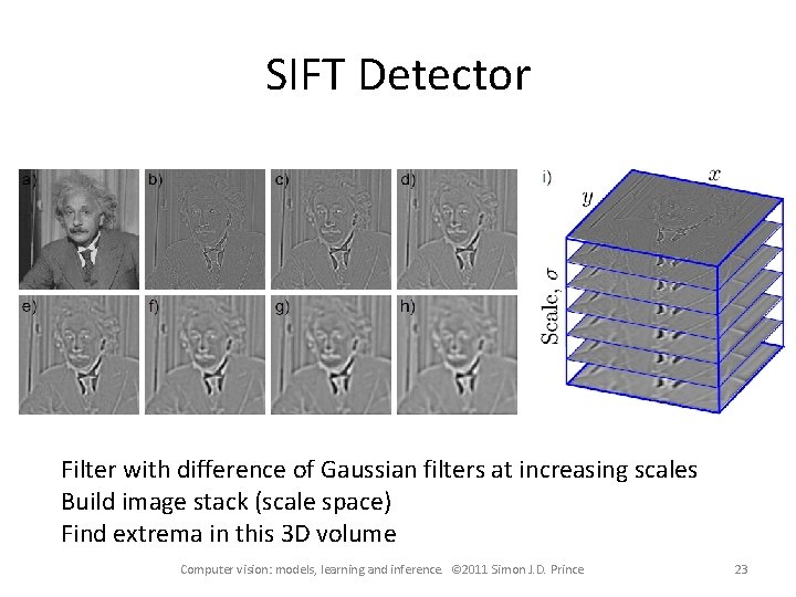
SIFT Detector Filter with difference of Gaussian filters at increasing scales Build image stack (scale space) Find extrema in this 3 D volume Computer vision: models, learning and inference. © 2011 Simon J. D. Prince 23

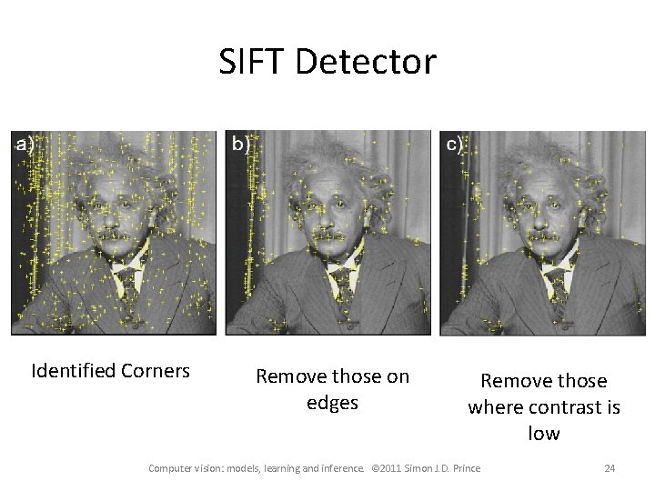
SIFT Detector Identified Corners Remove those on edges Remove those where contrast is low Computer vision: models, learning and inference. © 2011 Simon J. D. Prince 24

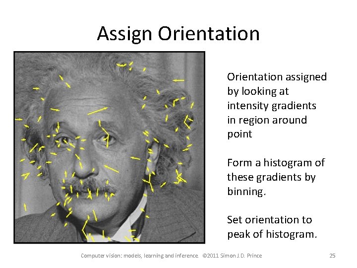
Assign Orientation assigned by looking at intensity gradients in region around point Form a histogram of these gradients by binning. Set orientation to peak of histogram. Computer vision: models, learning and inference. © 2011 Simon J. D. Prince 25

Structure • • Per-pixel transformations Edges, corners, and interest points Descriptors Dimensionality reduction Computer vision: models, learning and inference. © 2011 Simon J. D. Prince 26

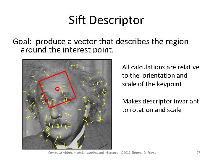
Sift Descriptor Goal: produce a vector that describes the region around the interest point. All calculations are relative to the orientation and scale of the keypoint Makes descriptor invariant to rotation and scale Computer vision: models, learning and inference. © 2011 Simon J. D. Prince 27

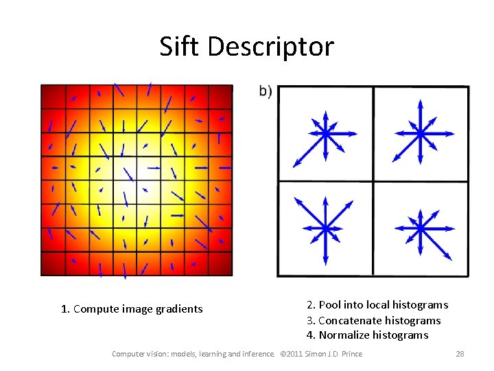
Sift Descriptor 1. Compute image gradients 2. Pool into local histograms 3. Concatenate histograms 4. Normalize histograms Computer vision: models, learning and inference. © 2011 Simon J. D. Prince 28

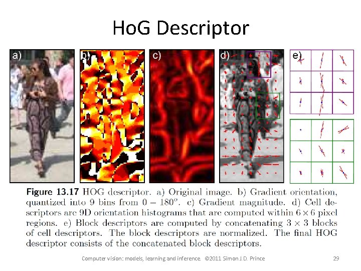
Ho. G Descriptor Computer vision: models, learning and inference. © 2011 Simon J. D. Prince 29

Bag of words descriptor • • • Compute visual features in image Compute descriptor around each Find closest match in library and assign index Compute histogram of these indices over the region Dictionary computed using K-means Computer vision: models, learning and inference. © 2011 Simon J. D. Prince 30

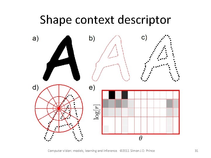
Shape context descriptor Computer vision: models, learning and inference. © 2011 Simon J. D. Prince 31

Structure • • Per-pixel transformations Edges, corners, and interest points Descriptors Dimensionality reduction Computer vision: models, learning and inference. © 2011 Simon J. D. Prince 32

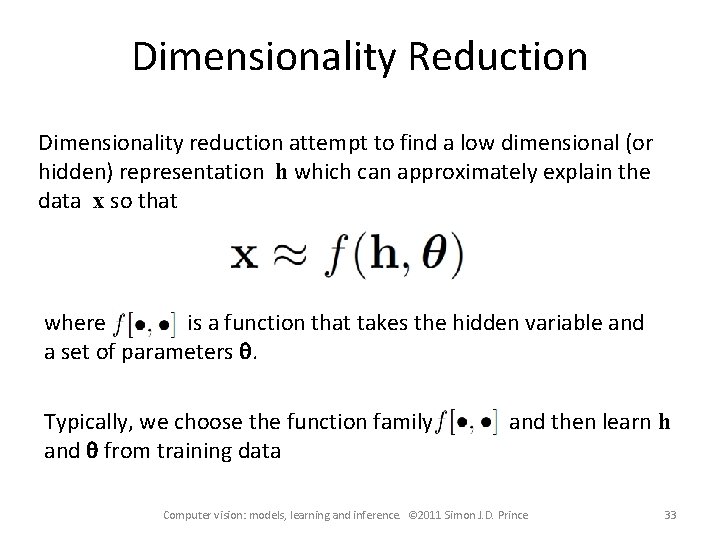
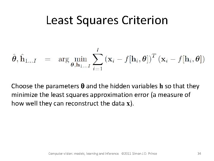
Dimensionality Reduction Dimensionality reduction attempt to find a low dimensional (or hidden) representation h which can approximately explain the data x so that where is a function that takes the hidden variable and a set of parameters q. Typically, we choose the function family and q from training data and then learn h Computer vision: models, learning and inference. © 2011 Simon J. D. Prince 33

Least Squares Criterion Choose the parameters q and the hidden variables h so that they minimize the least squares approximation error (a measure of how well they can reconstruct the data x). Computer vision: models, learning and inference. © 2011 Simon J. D. Prince 34

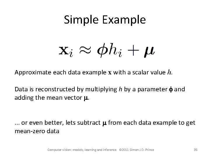
Simple Example Approximate each data example x with a scalar value h. Data is reconstructed by multiplying h by a parameter f and adding the mean vector m. . or even better, lets subtract m from each data example to get mean-zero data Computer vision: models, learning and inference. © 2011 Simon J. D. Prince 35

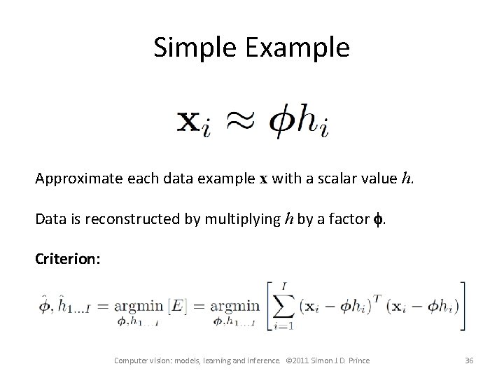
Simple Example Approximate each data example x with a scalar value h. Data is reconstructed by multiplying h by a factor f. Criterion: Computer vision: models, learning and inference. © 2011 Simon J. D. Prince 36

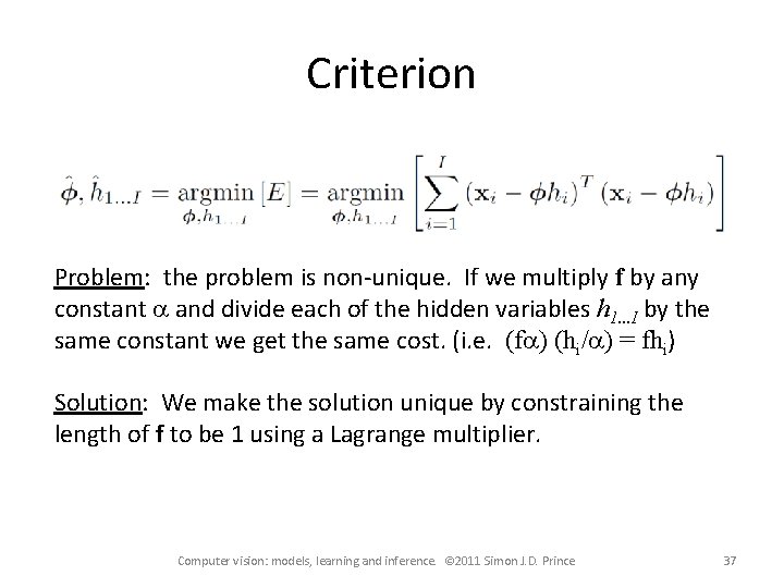
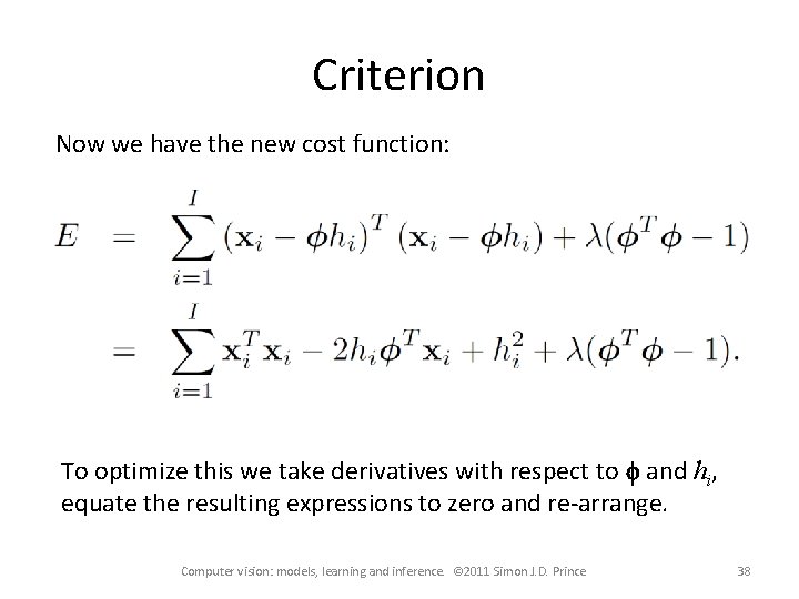
Criterion Problem: the problem is non-unique. If we multiply f by any constant a and divide each of the hidden variables h 1. . . I by the same constant we get the same cost. (i. e. (fa) (hi/a) = fhi) Solution: We make the solution unique by constraining the length of f to be 1 using a Lagrange multiplier. Computer vision: models, learning and inference. © 2011 Simon J. D. Prince 37

Criterion Now we have the new cost function: To optimize this we take derivatives with respect to f and hi, equate the resulting expressions to zero and re-arrange. Computer vision: models, learning and inference. © 2011 Simon J. D. Prince 38

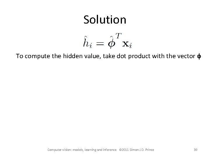
Solution To compute the hidden value, take dot product with the vector f Computer vision: models, learning and inference. © 2011 Simon J. D. Prince 39

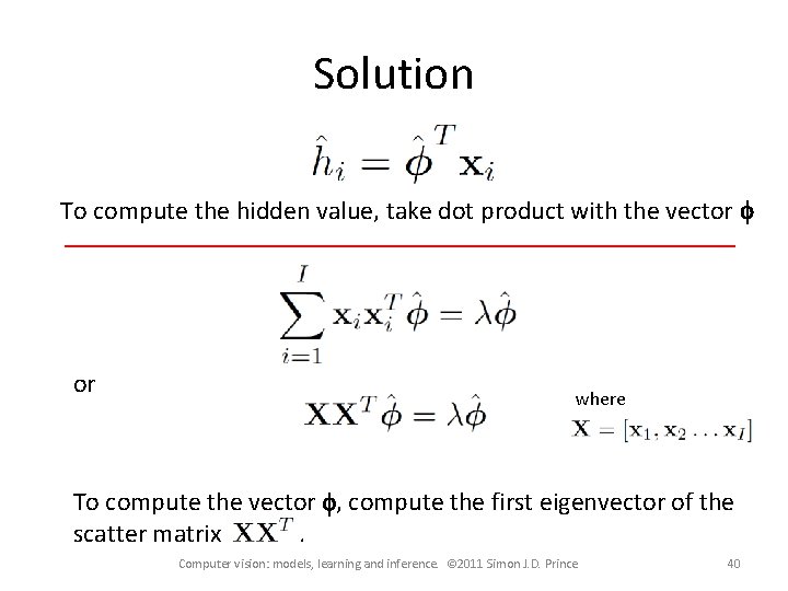
Solution To compute the hidden value, take dot product with the vector f or where To compute the vector f, compute the first eigenvector of the scatter matrix. Computer vision: models, learning and inference. © 2011 Simon J. D. Prince 40

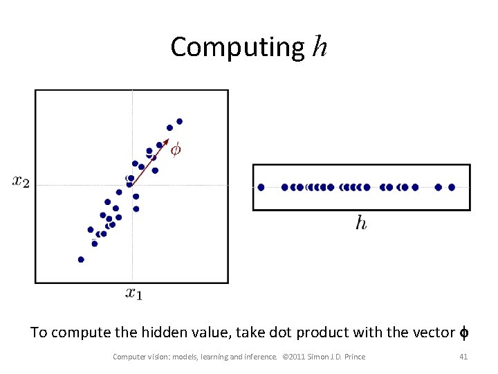
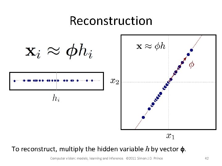
Computing h To compute the hidden value, take dot product with the vector f Computer vision: models, learning and inference. © 2011 Simon J. D. Prince 41

Reconstruction To reconstruct, multiply the hidden variable h by vector f. Computer vision: models, learning and inference. © 2011 Simon J. D. Prince 42

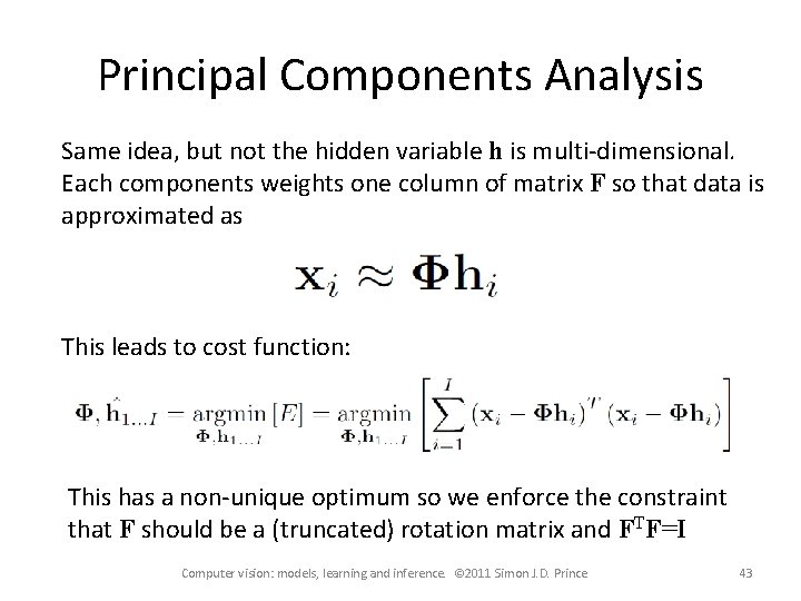
Principal Components Analysis Same idea, but not the hidden variable h is multi-dimensional. Each components weights one column of matrix F so that data is approximated as This leads to cost function: This has a non-unique optimum so we enforce the constraint that F should be a (truncated) rotation matrix and FTF=I Computer vision: models, learning and inference. © 2011 Simon J. D. Prince 43

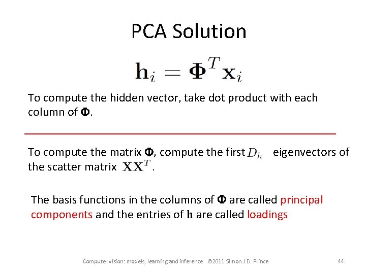
PCA Solution To compute the hidden vector, take dot product with each column of F. To compute the matrix F, compute the first the scatter matrix. eigenvectors of The basis functions in the columns of F are called principal components and the entries of h are called loadings Computer vision: models, learning and inference. © 2011 Simon J. D. Prince 44

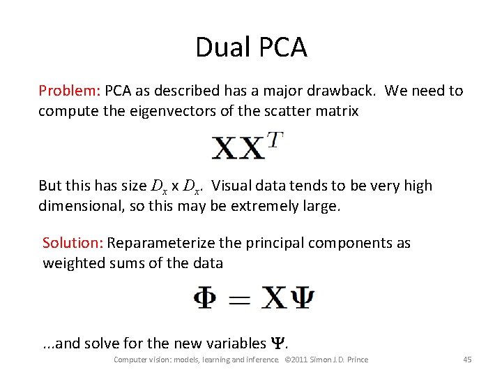
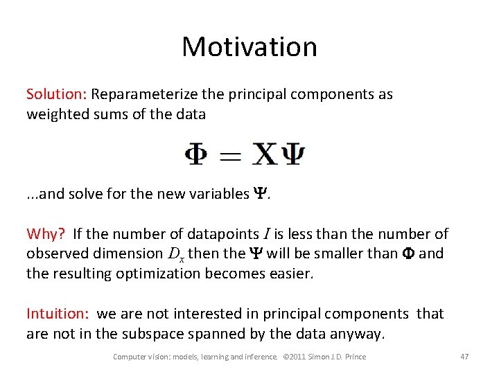
Dual PCA Problem: PCA as described has a major drawback. We need to compute the eigenvectors of the scatter matrix But this has size Dx x Dx. Visual data tends to be very high dimensional, so this may be extremely large. Solution: Reparameterize the principal components as weighted sums of the data . . . and solve for the new variables Y. Computer vision: models, learning and inference. © 2011 Simon J. D. Prince 45

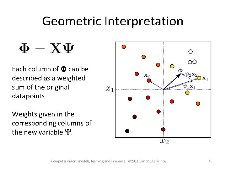
Geometric Interpretation Each column of F can be described as a weighted sum of the original datapoints. Weights given in the corresponding columns of the new variable Y. Computer vision: models, learning and inference. © 2011 Simon J. D. Prince 46

Motivation Solution: Reparameterize the principal components as weighted sums of the data . . . and solve for the new variables Y. Why? If the number of datapoints I is less than the number of observed dimension Dx then the Y will be smaller than F and the resulting optimization becomes easier. Intuition: we are not interested in principal components that are not in the subspace spanned by the data anyway. Computer vision: models, learning and inference. © 2011 Simon J. D. Prince 47

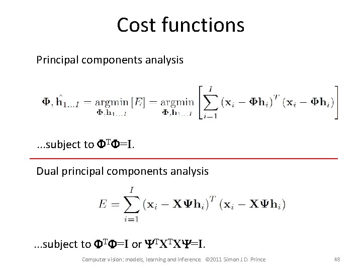
Cost functions Principal components analysis . . . subject to FTF=I. Dual principal components analysis . . . subject to FTF=I or YTXTXY=I. Computer vision: models, learning and inference. © 2011 Simon J. D. Prince 48

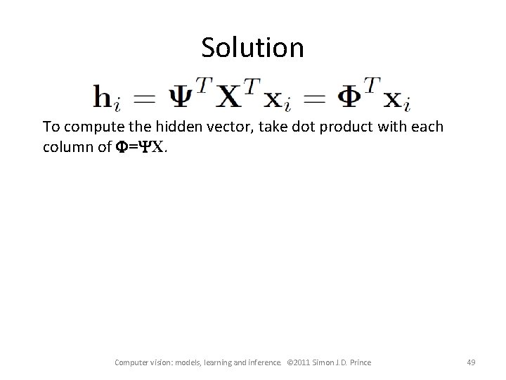
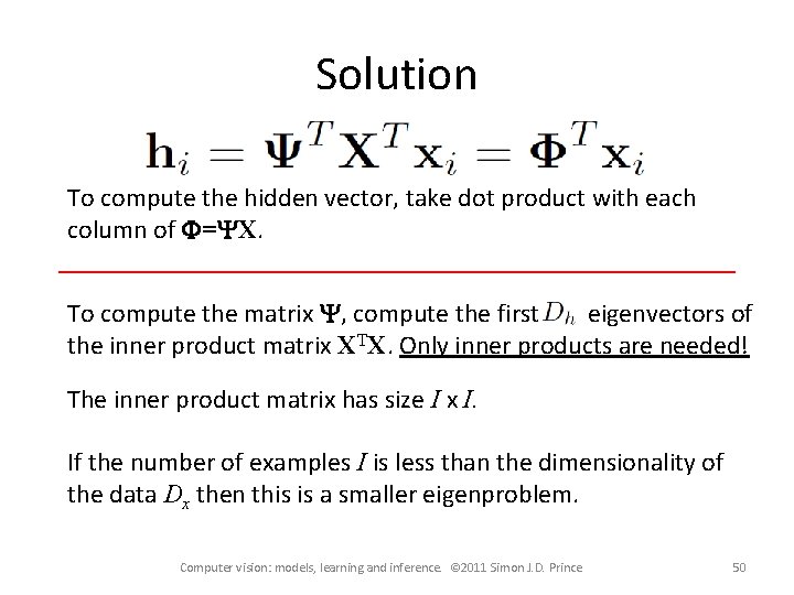
Solution To compute the hidden vector, take dot product with each column of F=YX. Computer vision: models, learning and inference. © 2011 Simon J. D. Prince 49

Solution To compute the hidden vector, take dot product with each column of F=YX. To compute the matrix Y, compute the first eigenvectors of the inner product matrix XTX. Only inner products are needed! The inner product matrix has size I x I. If the number of examples I is less than the dimensionality of the data Dx then this is a smaller eigenproblem. Computer vision: models, learning and inference. © 2011 Simon J. D. Prince 50

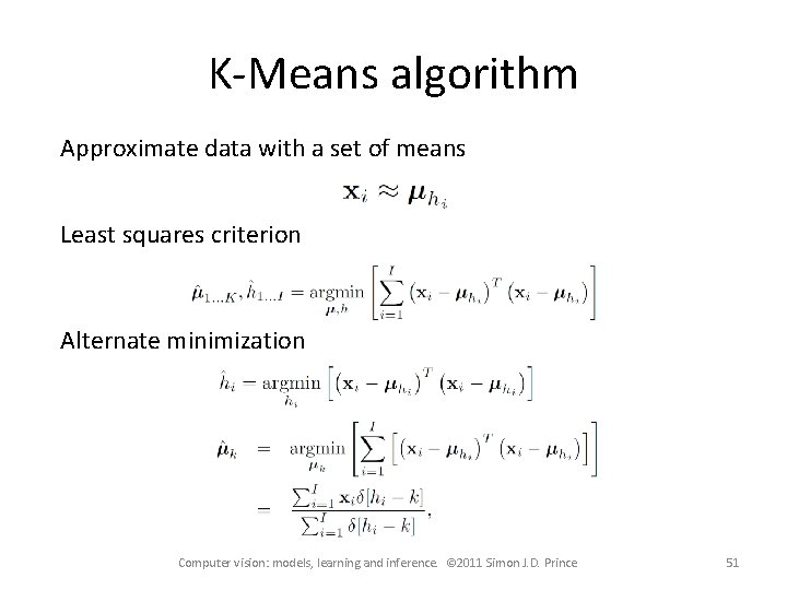
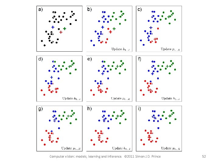
K-Means algorithm Approximate data with a set of means Least squares criterion Alternate minimization Computer vision: models, learning and inference. © 2011 Simon J. D. Prince 51

Computer vision: models, learning and inference. © 2011 Simon J. D. Prince 52