Parallel Computer Models THE STATE OF COMPUTING Computer


 2. SIMD (single")


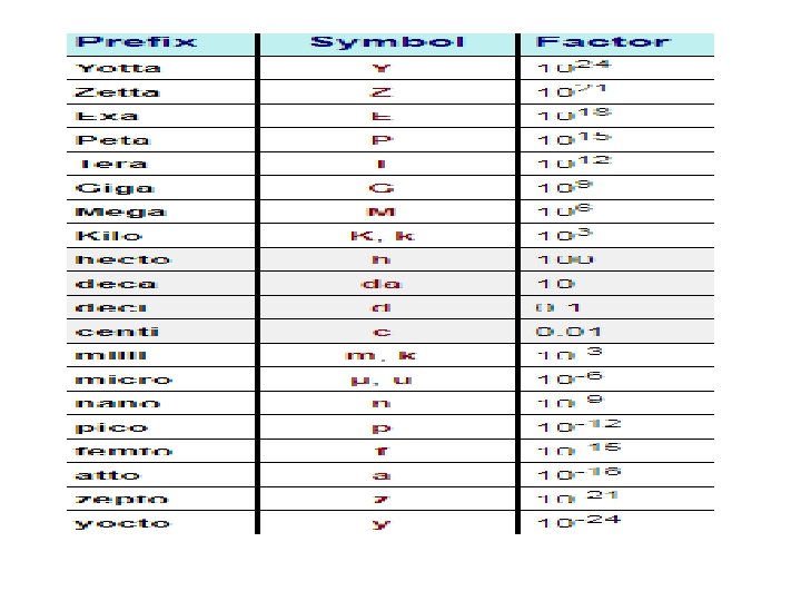
 • gflops, • teraflops or • petaflops.")


- Slides: 70
Parallel Computer Models
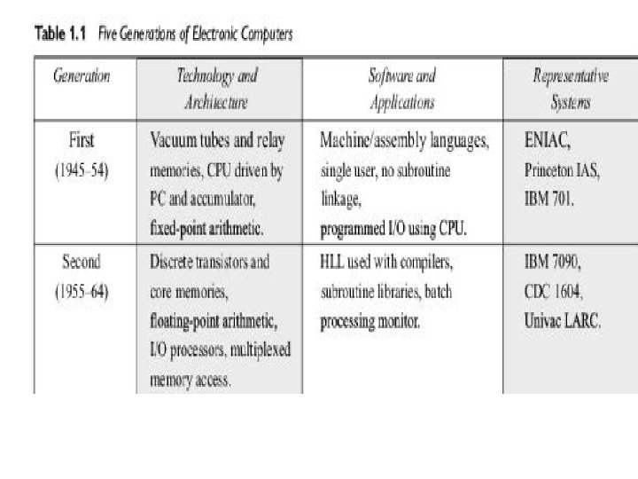
THE STATE OF COMPUTING Computer Development Milestones • Prior to I 945, computers were made with mechanical or electromechanical pans. • The earliest mechanical computer can be traced back to 5110 BC in the form of the abacus used in China. The abacus is manually operated to perform decimal arithmetic with carry Propagation digit by digit. • Blaise Pascal built a mechanical adder and subtractor in France in 1642. Charles Babbage designed a difference engine in England for polynomial evaluation in 1827. • Konrad Zuse built the first binary mechanical computer in Germany in 1941. • Howard Aiken proposed the very first electromechanical decimal computer, which was built as the Harvard Mark I by IBM in 1944. • Both Zuse’s and Aiken‘s machines were designed for generalpurpose computations.
• 1 Million = 10 Lakhs = 1 followed by 6 Zeros = 1, 000 • 10 Million = 1 Crore • 100 Million = 10 crore • 1000 Million = 100 Crore = 1 Billion
Elements of Modern Computers
Evolution of Computer Architecture
Flynn’s classification 1. SISD(single instruction stream over a single data stream) 2. SIMD (single instruction stream over a multiple data stream) 3. MIMD(multiple instruction stream over a multiple data stream) 4. MISD(multiple instruction stream over a single data stream)
Flynn’s classification • Of the four machine models, most parallel computers built in the past assumed the MIMD model for general purpose computations. • The SIMD and MISD models are more suitable for special-purpose computations. • For this reason, MIMD is the most popular model, SIMD next, and MISD the least popular model being applied in commercial machines
Development Layers
System Attributes affecting Performance • The ideal performance of a computer system demands a perfect match between 1. Machine capability 2. Program behavior.
System Attributes affecting Performance • Machine capability can be enhanced with better hardware technology, innovative architectural features, and efficient resources management. • However, program behavior is difficult to predict due to its heavy dependence on application and run-time conditions
System Attributes affecting Performance • There also many other factors affecting program behavior, including 1. Algorithm design, 2. Data structures, 3. Language efficiency, 4. Programmer skill, and 5. Compiler technology
System Attributes affecting Performance • The simplest measure of program performance is the turnaround time?
System Attributes affecting Performance • The simplest measure of program performance is the turnaround time which includes 1. disk and memory accesses, 2. input and output activities, 3. compilation time, 4. OS overhead, and 5. CPU time
System Attributes affecting Performance Clock Rate and CPI • The CPU of today‘s digital computer is driven by a clock with a constant cycle time T • The inverse of the cycle time is the clock rate (f= 1/T).
CPU Performance © Essentially all computers are constructed using clock (all called ticks, clock periods, clocks, cycles, or clock cycles) running at a constant rate. u u Clock rate: today in GHz Clock cycle time: clock cycle time = 1/clock rate © Thus, the CPU time for a program can be expressed two ways: 1 Or, 2 Computer Architecture- 23
CPU Performance © We can also count the number of instructions executed – the instruction path length or instruction count (IC). © If we know the number of clock cycles and IC, then the average number of clock cycles per instruction (CPI). © CPI is computed as 3 © Thus, clock cycles can be defined as IC × CPI, this allows us to use CPI in the execution time formula: Substituting Equation 3 in Equation 1 we get 4 Computer Architecture- 24
CPU Performance © The pieces fit together of CPU time . † Processor performance is dependent upon three characteristics: instruction count, clock cycles per instruction and clock cycle (or rate). Computer Architecture- 25
System Attributes affecting Performance
System attributes
Problem 1
Problem 1 Solution
Problem 2
Problem 2 solution
Problem 3 Determine CPI and execution time for this program
MIPS rate • The processor speed is often measured in terms of million instructions per second (MIPS). • Let C be the total number of clock cycles and T be cpu time needed to execute a given program • MIPS rate varies with respect to a number of factors, including the clock rate , the instruction count and the CPI of a given machine
Floating Point Operations per Second(flops) • gflops, • teraflops or • petaflops.
Programming Environments • Implicit Parallelism • Explicit Parallelism
Programming Environments • Implicit Parallelism:
Problem 4 • You are on the design team for a new processor. The clock of the processor runs at 200 MHz. The following table gives instruction frequencies for Benchmark B, as well as how many cycles the instructions take, for the different classes of instructions. For this problem, we assume that (unlike many of today's computers) the processor only executes one instruction at a time. Instruction Type Frequency Cycles Loads & Stores 30% 6 cycles Arithmetic Instructions 50% 4 cycles All Others 20% 3 cycles Calculate the CPI for Benchmark B.
Problem 4 solution • If we say that there are 100 instructions, then: 30 of them will be loads and stores. 50 of them will be arithmetic instructions. 20 of them will be all others. (30 * 6) + (50 * 4) + (20 * 3) = 440 cycles/100 instructions Therefore, there are 4. 4 Cycles per instruction.
Problem 4 • Suppose we have two implementations of the same instruction set architecture. Computer A has a clock cycle time of 250 ps and a CPI of 2. 0 for some program, and computer B has a clock cycle time of 500 ps and a CPI of 1. 2 for the same program. Which computer is faster for this program and by how much?
Solution
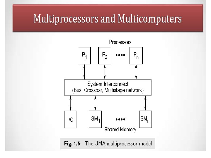
NUMA Model
COMA Model
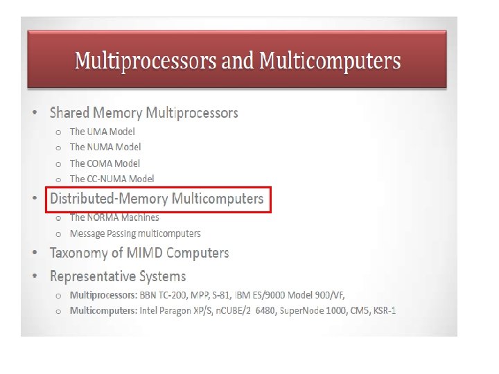
Distributed memory multicomputers
Taxonomy of MIMD Computers
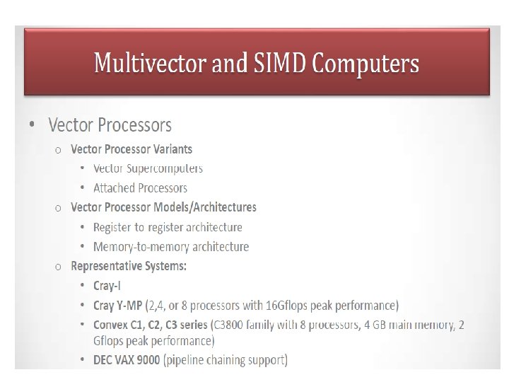
Vector Super. Computer
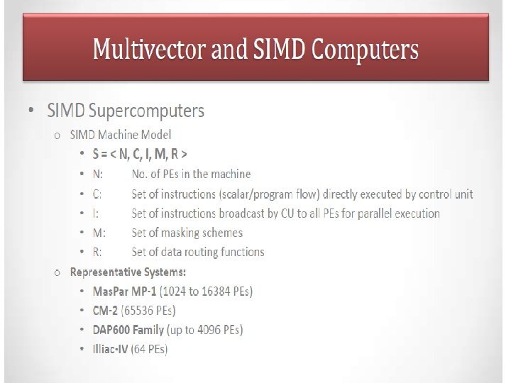
SIMD Computers
Program and Network Properties • CONDITIONS OF PARALLELISM Data and Resource Dependence: • The ordering relationship between statements indicated by the data dependence. Five types of data dependence are defined below 1. Flow dependence 2. Antidependence 3. Output dependence 4. I/O dependence 5. Unknown dependence
Program and Network Properties
Program and Network Properties
Problem 1 • Perform a data dependence analysis on each of the following Fortran program fragments. Show the dependence graphs among the statements with justification
Problem 1 • Perform a data dependence analysis on each of the following Fortran program fragments. Show the dependence graphs among the statements with justification
Problem 2 • Perform a data dependence analysis on each of the following Fortran program fragments. Show the dependence graphs among the statements with justification
Problem 2 • Perform a data dependence analysis on each of the following Fortran program fragments. Show the dependence graphs among the statements with justification
Control Dependence
Bernstein’s Condition These three conditions are known as Bernstein’s Condition.
Detection of parallelism in a program using Bernstein's conditions • Consider the simple case in which each process is a single HLL statement. We want to detect the parallelism embedded in the following five statements labeled PI, P 2, P 3, P 4, and P 5 in program order
Detection of parallelism in a program using Bernstein's conditions
Detection of parallelism in a program using Bernstein's conditions
Detection of parallelism in a program using Bernstein's conditions
PROGRAM PARTITIOHI NG AND SCHEDULING • Grain Sizes and Latency