Computer vision models learning and inference Chapter 3

Computer vision: models, learning and inference Chapter 3 Common probability distributions

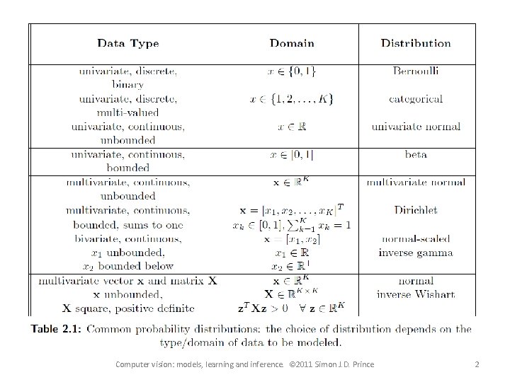
Computer vision: models, learning and inference. © 2011 Simon J. D. Prince 2

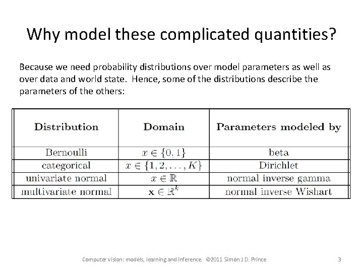
Why model these complicated quantities? Because we need probability distributions over model parameters as well as over data and world state. Hence, some of the distributions describe the parameters of the others: Computer vision: models, learning and inference. © 2011 Simon J. D. Prince 3

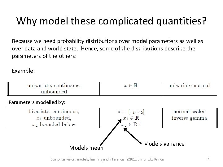
Why model these complicated quantities? Because we need probability distributions over model parameters as well as over data and world state. Hence, some of the distributions describe the parameters of the others: Example: Parameters modelled by: Models mean Models variance Computer vision: models, learning and inference. © 2011 Simon J. D. Prince 4

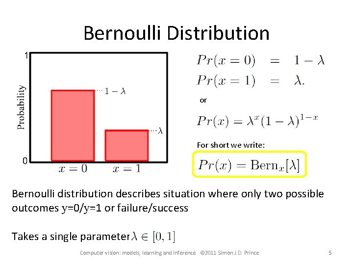
Bernoulli Distribution or For short we write: Bernoulli distribution describes situation where only two possible outcomes y=0/y=1 or failure/success Takes a single parameter Computer vision: models, learning and inference. © 2011 Simon J. D. Prince 5

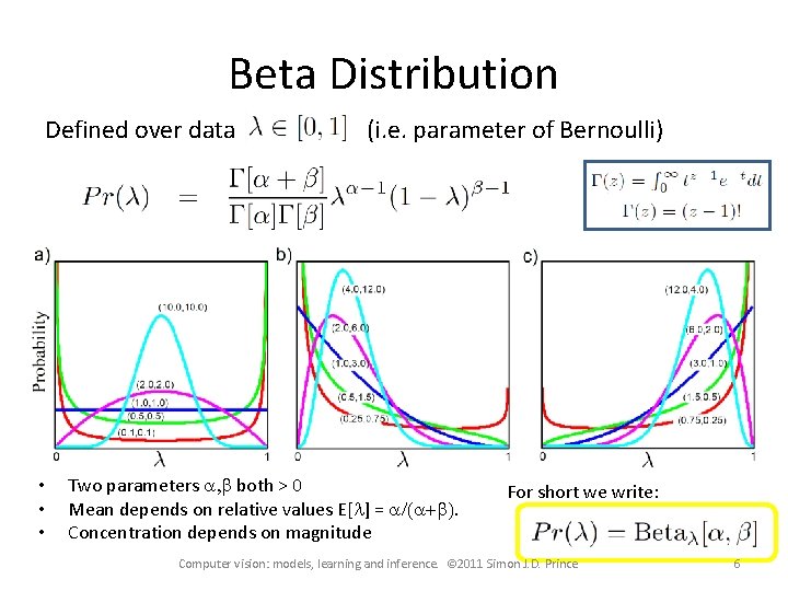
Beta Distribution Defined over data • • • (i. e. parameter of Bernoulli) Two parameters a, b both > 0 Mean depends on relative values E[l] = a/(a+b). Concentration depends on magnitude For short we write: Computer vision: models, learning and inference. © 2011 Simon J. D. Prince 6

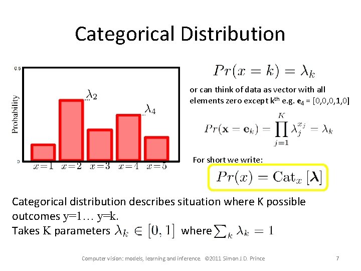
Categorical Distribution or can think of data as vector with all elements zero except kth e. g. e 4 = [0, 0, 0, 1, 0] For short we write: Categorical distribution describes situation where K possible outcomes y=1… y=k. Takes K parameters where Computer vision: models, learning and inference. © 2011 Simon J. D. Prince 7

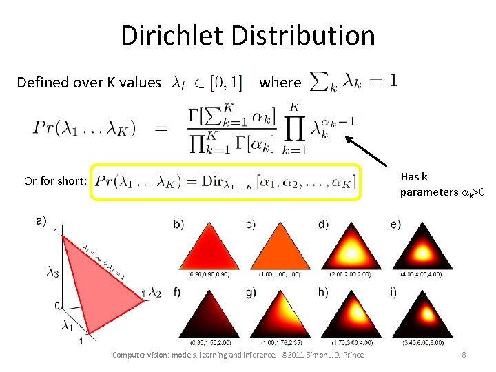
Dirichlet Distribution Defined over K values where Has k parameters ak>0 Or for short: Computer vision: models, learning and inference. © 2011 Simon J. D. Prince 8

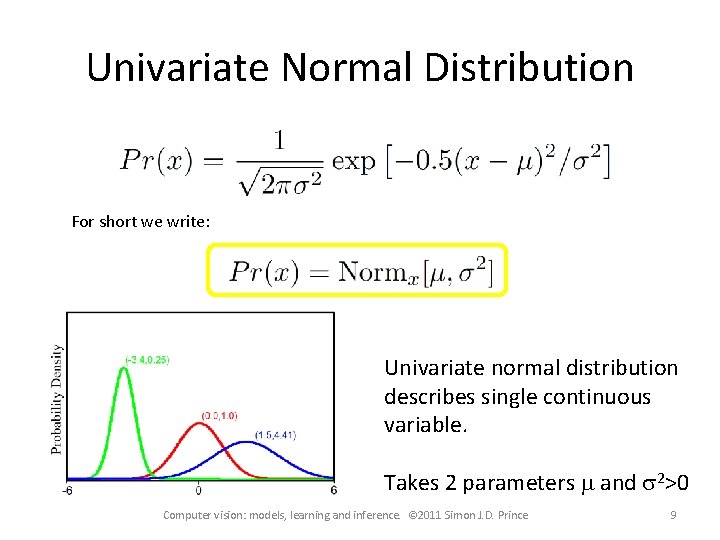
Univariate Normal Distribution For short we write: Univariate normal distribution describes single continuous variable. Takes 2 parameters m and s 2>0 Computer vision: models, learning and inference. © 2011 Simon J. D. Prince 9

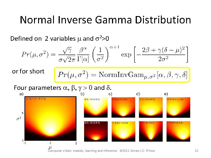
Normal Inverse Gamma Distribution Defined on 2 variables m and s 2>0 or for short Four parameters a, b, g > 0 and d. Computer vision: models, learning and inference. © 2011 Simon J. D. Prince 10

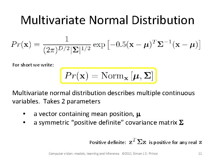
Multivariate Normal Distribution For short we write: Multivariate normal distribution describes multiple continuous variables. Takes 2 parameters • • a vector containing mean position, m a symmetric “positive definite” covariance matrix S Positive definite: is positive for any real Computer vision: models, learning and inference. © 2011 Simon J. D. Prince 11

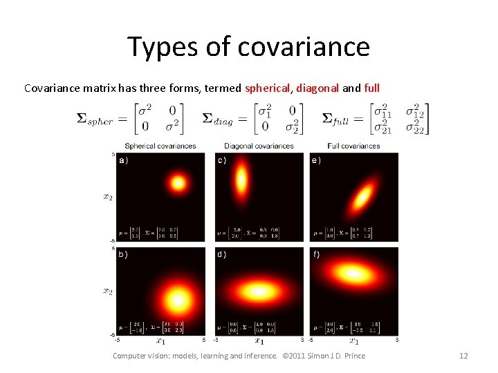
Types of covariance Covariance matrix has three forms, termed spherical, diagonal and full Computer vision: models, learning and inference. © 2011 Simon J. D. Prince 12

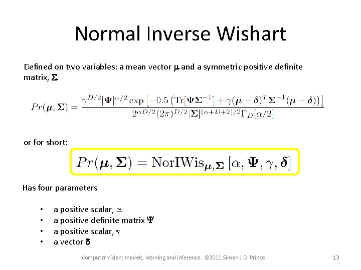
Normal Inverse Wishart Defined on two variables: a mean vector m and a symmetric positive definite matrix, S. or for short: Has four parameters • • a positive scalar, a a positive definite matrix Y a positive scalar, g a vector d Computer vision: models, learning and inference. © 2011 Simon J. D. Prince 13

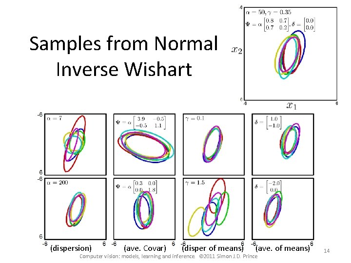
Samples from Normal Inverse Wishart (dispersion) (ave. Covar) (disper of means) (ave. of means) Computer vision: models, learning and inference. © 2011 Simon J. D. Prince 14

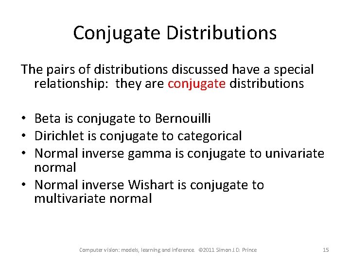
Conjugate Distributions The pairs of distributions discussed have a special relationship: they are conjugate distributions • Beta is conjugate to Bernouilli • Dirichlet is conjugate to categorical • Normal inverse gamma is conjugate to univariate normal • Normal inverse Wishart is conjugate to multivariate normal Computer vision: models, learning and inference. © 2011 Simon J. D. Prince 15

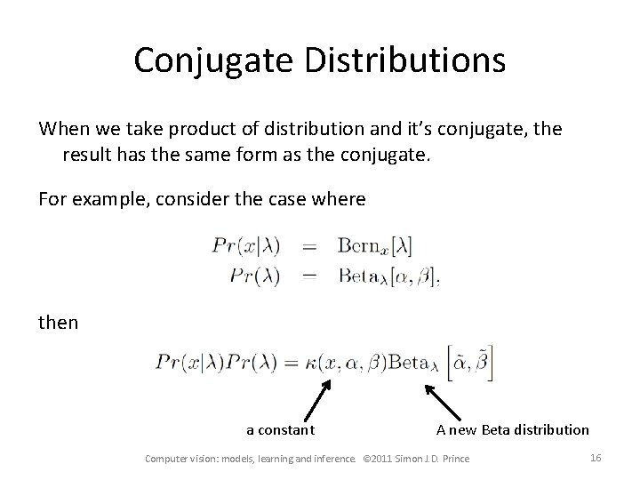
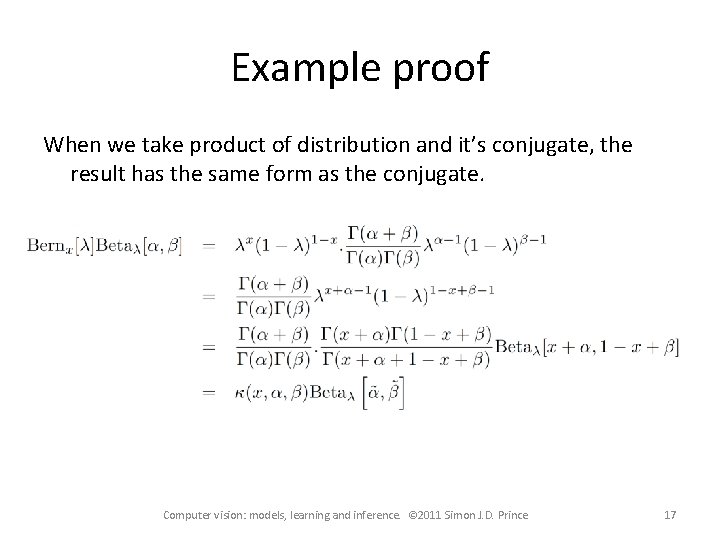
Conjugate Distributions When we take product of distribution and it’s conjugate, the result has the same form as the conjugate. For example, consider the case where then a constant A new Beta distribution Computer vision: models, learning and inference. © 2011 Simon J. D. Prince 16

Example proof When we take product of distribution and it’s conjugate, the result has the same form as the conjugate. Computer vision: models, learning and inference. © 2011 Simon J. D. Prince 17

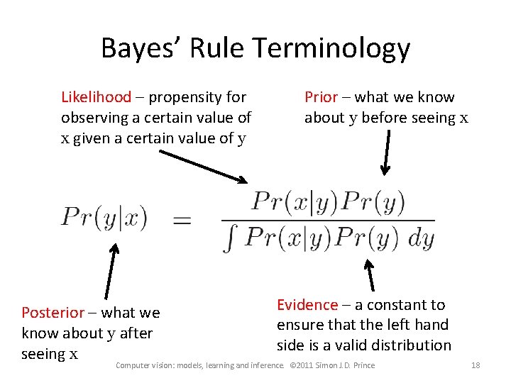
Bayes’ Rule Terminology Likelihood – propensity for observing a certain value of x given a certain value of y Posterior – what we know about y after seeing x Prior – what we know about y before seeing x Evidence – a constant to ensure that the left hand side is a valid distribution Computer vision: models, learning and inference. © 2011 Simon J. D. Prince 18

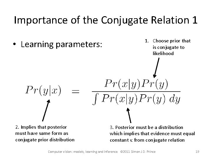
Importance of the Conjugate Relation 1 • Learning parameters: 2. Implies that posterior must have same form as conjugate prior distribution 1. Choose prior that is conjugate to likelihood 3. Posterior must be a distribution which implies that evidence must equal constant k from conjugate relation Computer vision: models, learning and inference. © 2011 Simon J. D. Prince 19

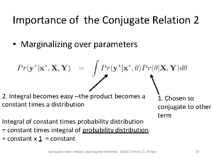
Importance of the Conjugate Relation 2 • Marginalizing over parameters 2. Integral becomes easy --the product becomes a constant times a distribution Integral of constant times probability distribution = constant times integral of probability distribution = constant x 1 = constant Computer vision: models, learning and inference. © 2011 Simon J. D. Prince 1. Chosen so conjugate to other term 20

Conclusions • Presented four distributions which model useful quantities • Presented four other distributions which model the parameters of the first four • They are paired in a special way – the second set is conjugate to the other • In the following material we’ll see that this relationship is very useful Computer vision: models, learning and inference. © 2011 Simon J. D. Prince 21