Computer Vision Segmentation 1 Computer Vision Segmentation the

Computer Vision Segmentation 1

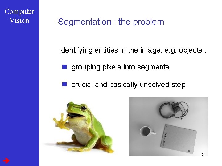
Computer Vision Segmentation : the problem Identifying entities in the image, e. g. objects : n grouping pixels into segments n crucial and basically unsolved step 2

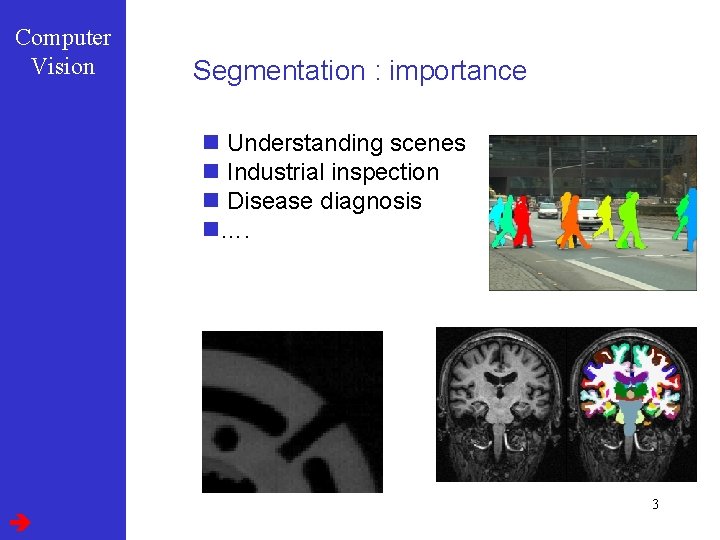
Computer Vision Segmentation : importance n Understanding scenes n Industrial inspection n Disease diagnosis n…. 3

Computer Vision Learning objectives: What can you do after today • Describe image segmentation task • Implement thresholding based techniques: – Morphological operators – Separating multiple components with region growing – Describe their limitations • Implement Hough transform to find lines, describe advantages and limitations • Describe different statistical pattern recognition based methods – Clustering – Supervised generative models – Discriminative learning principles 4

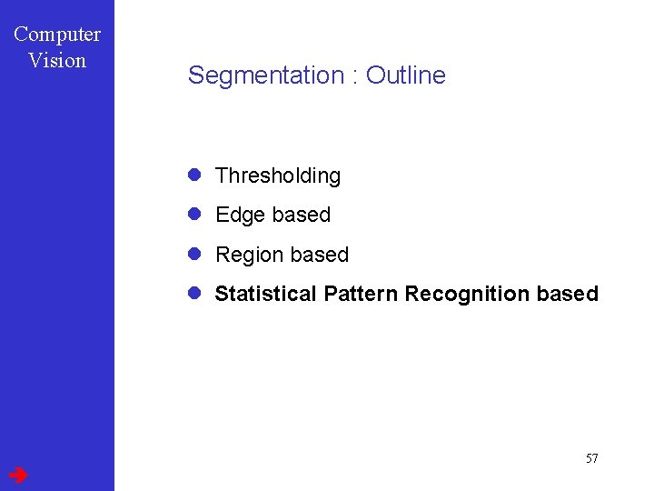
Computer Vision Segmentation : Outline l Thresholding l Edge based l Region based l Statistical Pattern Recognition based 5

Computer Vision Segmentation : Outline l Thresholding l Edge based l Region based l Statistical Pattern Recognition based 6

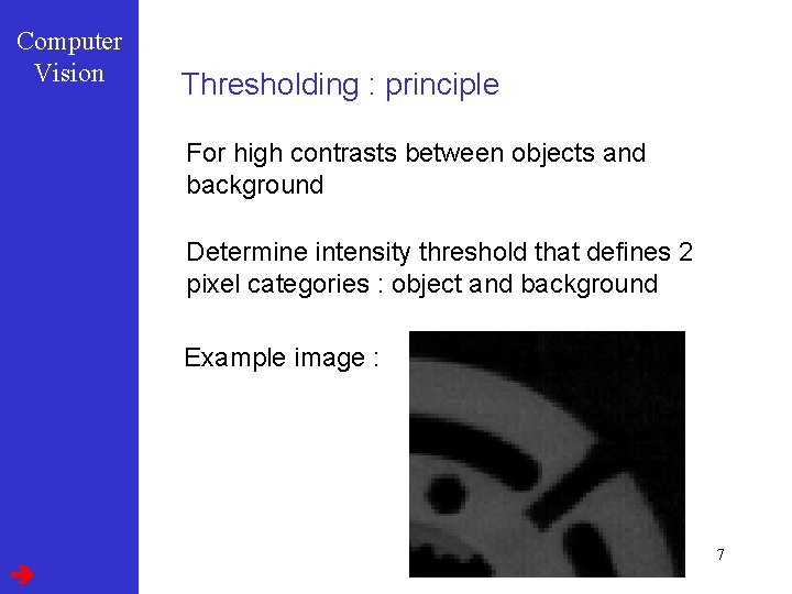
Computer Vision Thresholding : principle For high contrasts between objects and background Determine intensity threshold that defines 2 pixel categories : object and background Example image : 7

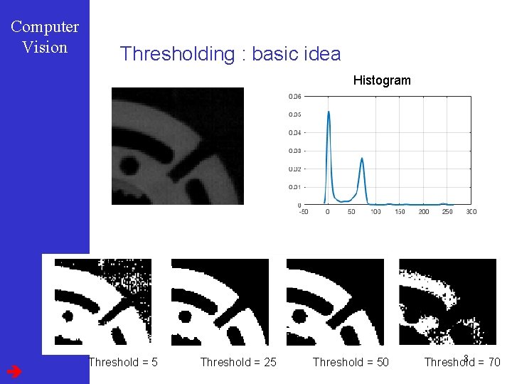
Computer Vision Thresholding : basic idea Histogram Threshold = 5 Threshold = 25 Threshold = 50 8 = 70 Threshold

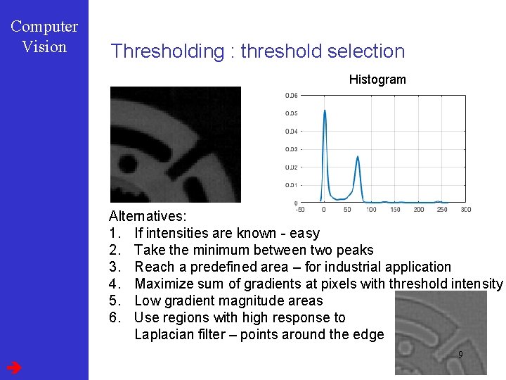
Computer Vision Thresholding : threshold selection Histogram Alternatives: 1. If intensities are known - easy 2. Take the minimum between two peaks 3. Reach a predefined area – for industrial application 4. Maximize sum of gradients at pixels with threshold intensity 5. Low gradient magnitude areas 6. Use regions with high response to Laplacian filter – points around the edge 9

Computer Vision Thresholding: Otsu criterion [Nobuyuki Otsu] Minimize within-group variance Group 1 I > threshold Otsu threshold = 35 Group 2 I <= threshold 10

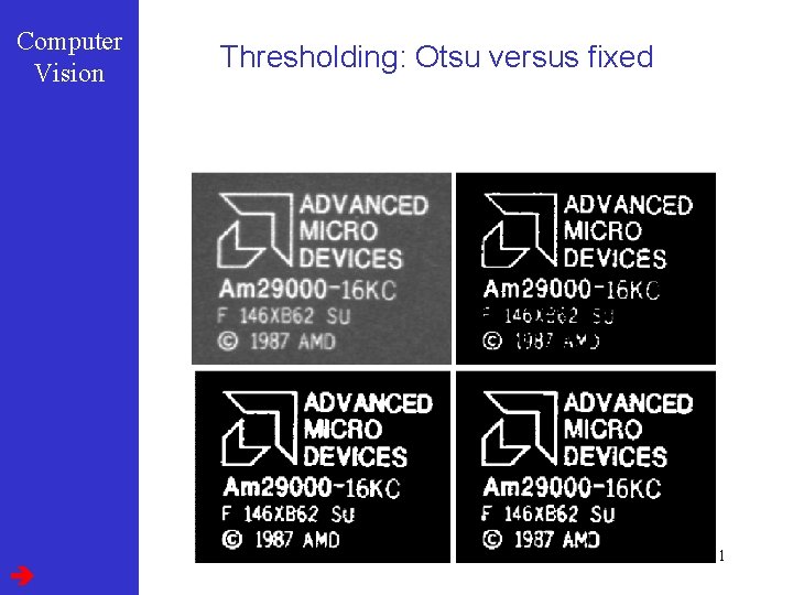
Computer Vision Thresholding: Otsu versus fixed Fixed threshold Image specific Otsu threshold Local Otsu threshold 11

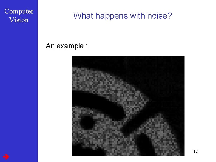
Computer Vision What happens with noise? An example : 12

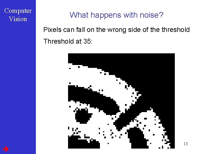
Computer Vision What happens with noise? Pixels can fall on the wrong side of the threshold Threshold at 35: 13

Computer Vision Solution: Enhancement of binary images Remove the isolated islands in the binary images Mathematical morphology 14

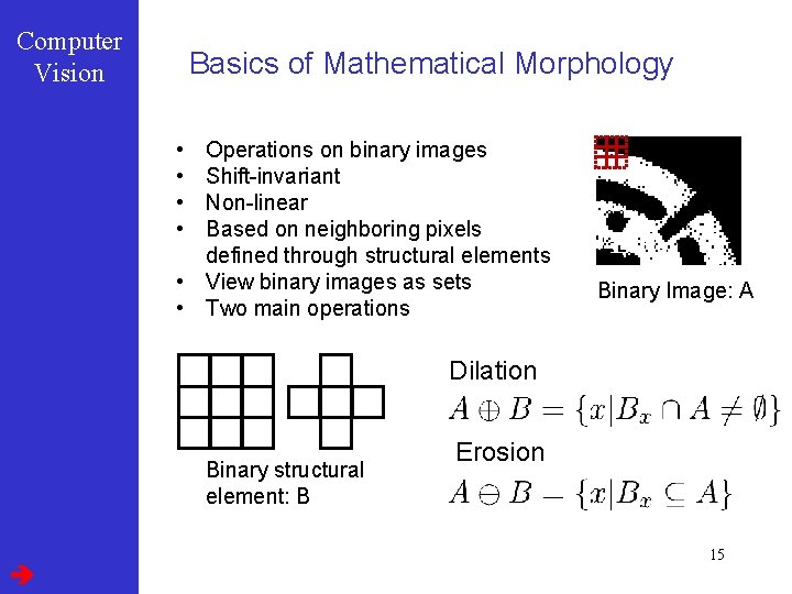
Computer Vision Basics of Mathematical Morphology • • Operations on binary images Shift-invariant Non-linear Based on neighboring pixels defined through structural elements • View binary images as sets • Two main operations Binary Image: A Dilation Binary structural element: B Erosion 15

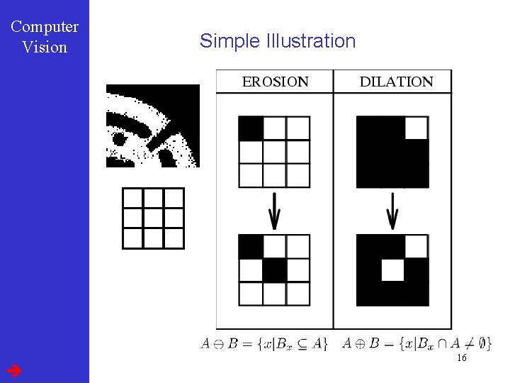
Computer Vision Simple Illustration 16

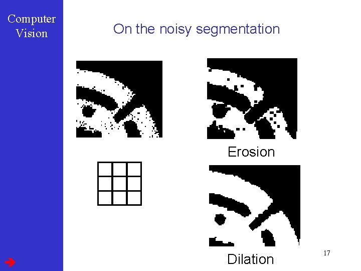
Computer Vision On the noisy segmentation Erosion Dilation 17

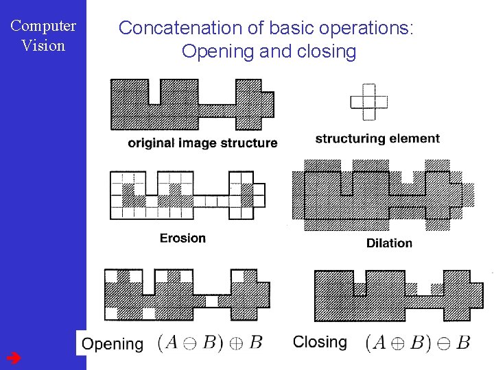
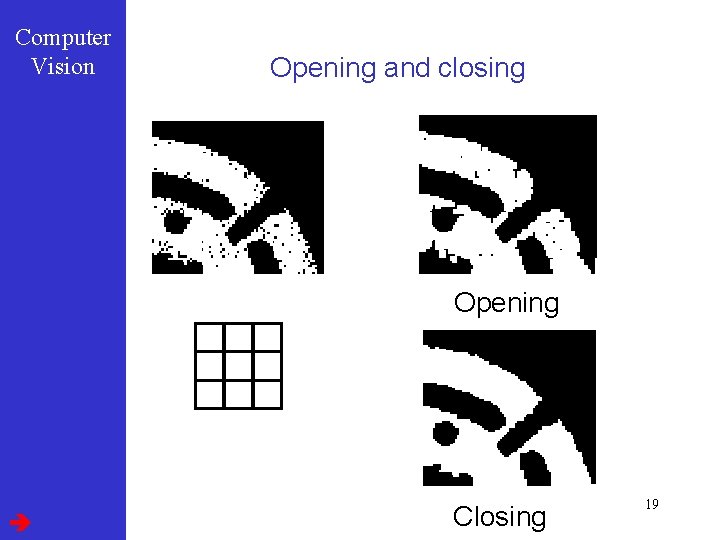
Computer Vision Concatenation of basic operations: Opening and closing

Computer Vision Opening and closing Opening Closing 19

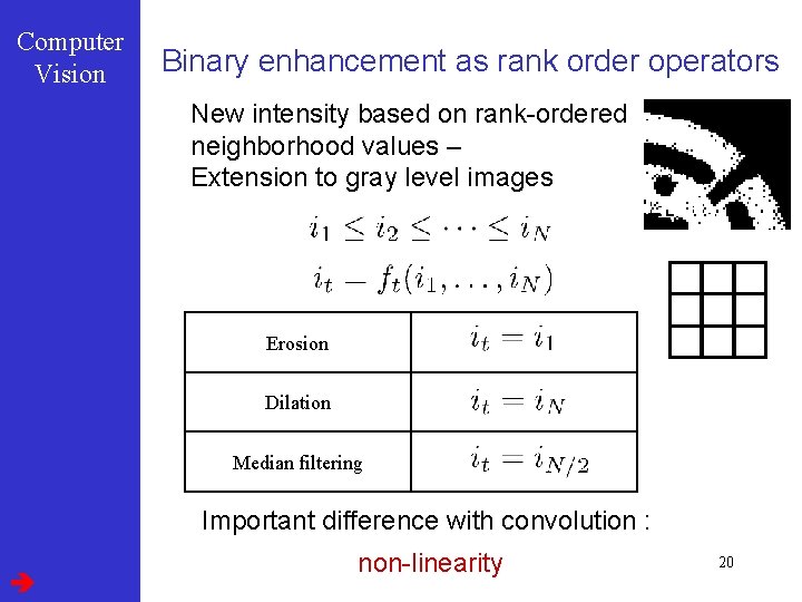
Computer Vision Binary enhancement as rank order operators New intensity based on rank-ordered neighborhood values – Extension to gray level images Erosion Dilation Median filtering Important difference with convolution : non-linearity 20

Computer Vision Binary enhancement : remarks n 1. Post-processing approach Many alternatives to enforce neighborhood consistency during segmentation n 2. Erosion + dilation (opening) Dilation + erosion (closing) n 3. Noise in background can be reduced by reversed operation n 4. Use same neighbourhood for both steps n 5. Reminder : median filtering useful for edge preserving smooting 21

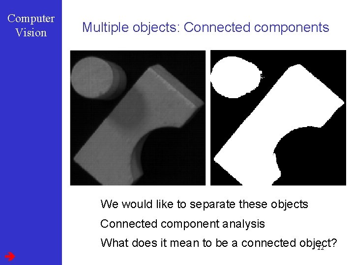
Computer Vision Multiple objects: Connected components We would like to separate these objects Connected component analysis What does it mean to be a connected object? 22

Computer Vision The structure of discrete image spaces Two main aspects • Topology • Distance Strong relationship 23

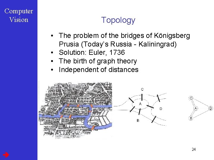
Computer Vision Topology • The problem of the bridges of Königsberg Prusia (Today’s Russia - Kaliningrad) • Solution: Euler, 1736 • The birth of graph theory • Independent of distances 24

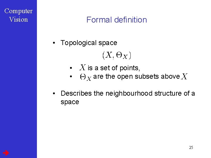
Computer Vision Formal definition • Topological space • • is a set of points, are the open subsets above • Describes the neighbourhood structure of a space 25

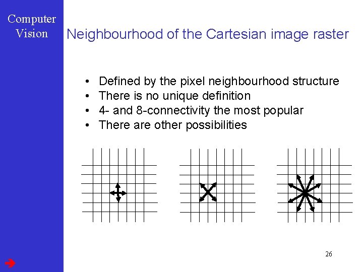
Computer Vision Neighbourhood of the Cartesian image raster • • Defined by the pixel neighbourhood structure There is no unique definition 4 - and 8 -connectivity the most popular There are other possibilities 26

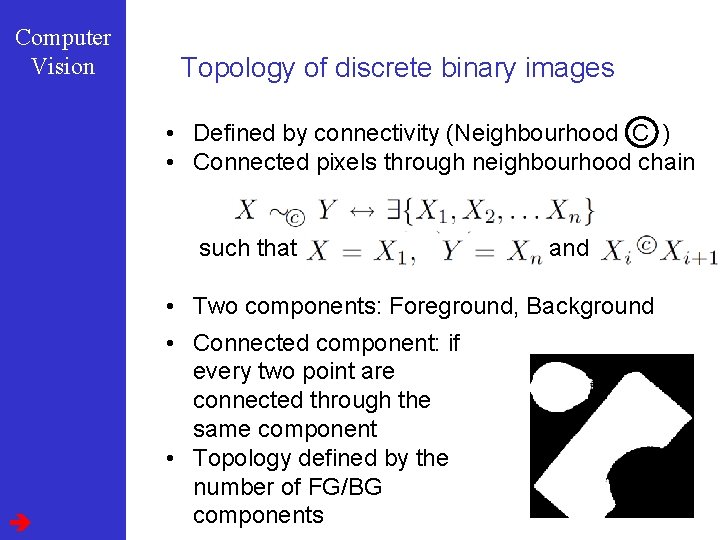
Computer Vision Topology of discrete binary images • Defined by connectivity (Neighbourhood C ) • Connected pixels through neighbourhood chain such that and • Two components: Foreground, Background • Connected component: if every two point are connected through the same component • Topology defined by the number of FG/BG components 27

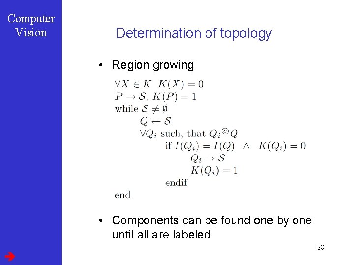
Computer Vision Determination of topology • Region growing • Components can be found one by one until all are labeled 28

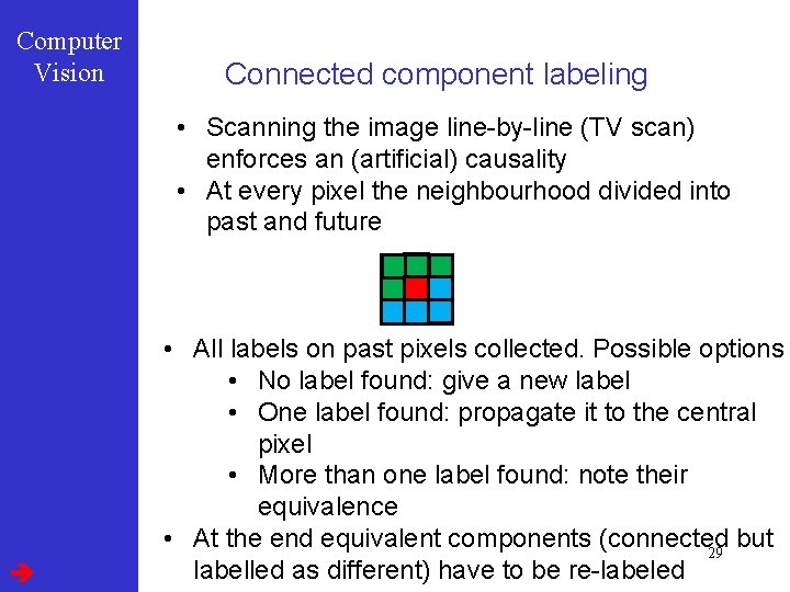
Computer Vision Connected component labeling • Scanning the image line-by-line (TV scan) enforces an (artificial) causality • At every pixel the neighbourhood divided into past and future • All labels on past pixels collected. Possible options • No label found: give a new label • One label found: propagate it to the central pixel • More than one label found: note their equivalence • At the end equivalent components (connected but 29 labelled as different) have to be re-labeled

Computer Vision 30

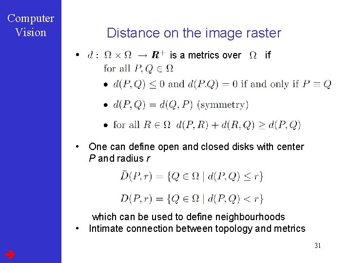
Computer Vision Distance on the image raster • is a metrics over if • One can define open and closed disks with center P and radius r which can be used to define neighbourhoods • Intimate connection between topology and metrics 31

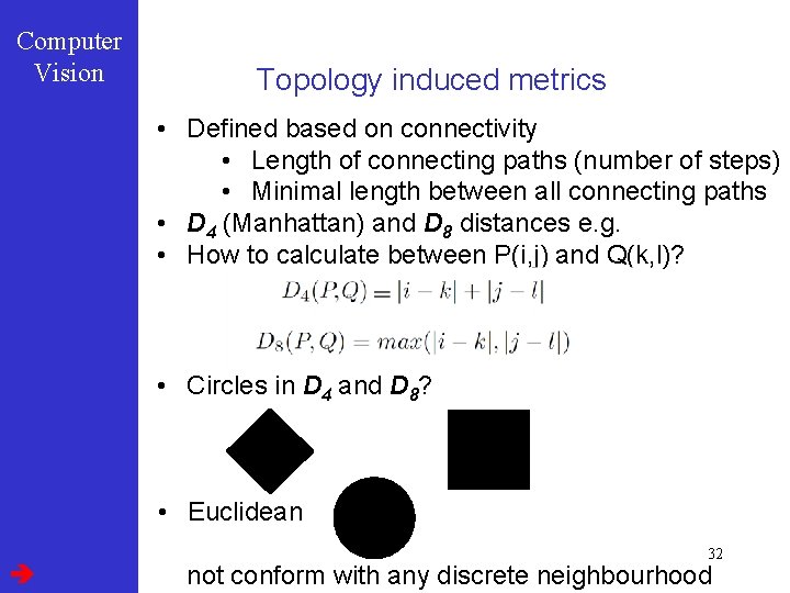
Computer Vision Topology induced metrics • Defined based on connectivity • Length of connecting paths (number of steps) • Minimal length between all connecting paths • D 4 (Manhattan) and D 8 distances e. g. • How to calculate between P(i, j) and Q(k, l)? • Circles in D 4 and D 8? • Euclidean 32 not conform with any discrete neighbourhood

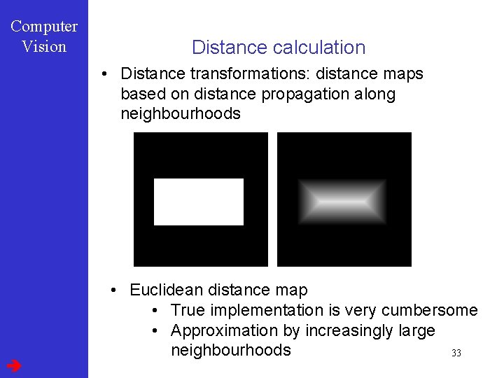
Computer Vision Distance calculation • Distance transformations: distance maps based on distance propagation along neighbourhoods • Euclidean distance map • True implementation is very cumbersome • Approximation by increasingly large neighbourhoods 33

Computer Vision Thresholding : remarks q Threshold advantages: 1. Serious bandwidth reduction 2. Simplification of further processing 3. Availability of real-time hardware for shape recognition q Generally it won’t provide a satisfying segmentation q Sometimes several thresholds yields finer labelling usually infeasible q Pixel-by-pixel decision • ignores neighbouring pixels • structural information lost 34

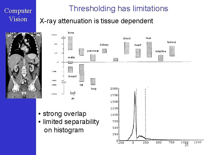
Computer Vision Thresholding has limitations X-ray attenuation is tissue dependent bone liver blood kidney pancreas tumour heart intestine water breast fat lung air • strong overlap • limited separability on histogram 35

Computer Vision Segmentation : Outline l Thresholding l Edge based l Region based l Statistical Pattern Recognition based 36

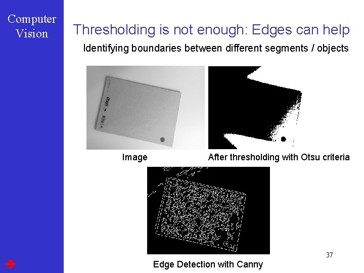
Computer Vision Thresholding is not enough: Edges can help Identifying boundaries between different segments / objects Image After thresholding with Otsu criteria 37 Edge Detection with Canny

Computer Vision Edge linking techniques l 1. Hough Transform: for predefined shapes l 2. Elastically deformable contour models Snakes: generic shape priors [Next week] l 3. Many other methods for grouping combination with user interaction (dynamic path search – in the script) 38

Computer Vision The Hough transform : principle Uses parametric shape models to extract objects in lower dimensional spaces In other words, if you know the shape, then Hough Transform can be used to detect it. The simplest example: straight lines Many further possibilities, like circles, ellipses and generalizations to other shapes 39

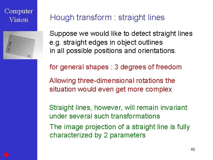
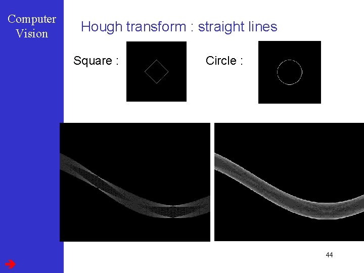
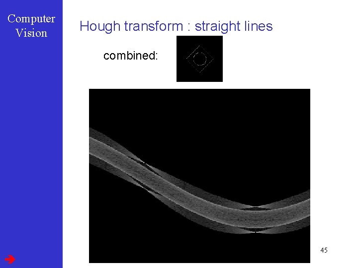
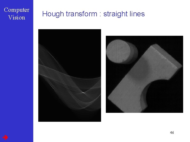
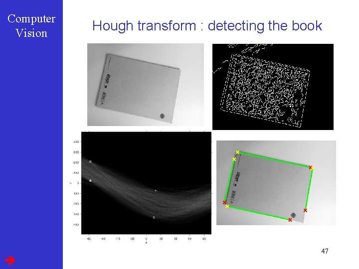
Computer Vision Hough transform : straight lines Suppose we would like to detect straight lines e. g. straight edges in object outlines in all possible positions and orientations. for general shapes : 3 degrees of freedom Allowing three-dimensional rotations the situation would even get more complex Straight lines, however, will remain invariant under several such transformations The image projection of a straight line is fully characterized by 2 parameters 40

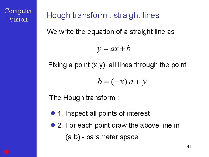
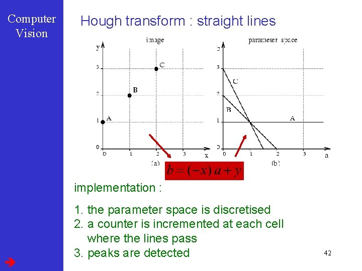
Computer Vision Hough transform : straight lines We write the equation of a straight line as Fixing a point (x, y), all lines through the point : The Hough transform : l 1. Inspect all points of interest l 2. For each point draw the above line in (a, b) - parameter space 41

Computer Vision Hough transform : straight lines implementation : 1. the parameter space is discretised 2. a counter is incremented at each cell where the lines pass 3. peaks are detected 42

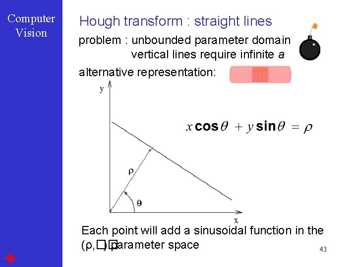
Computer Vision Hough transform : straight lines problem : unbounded parameter domain vertical lines require infinite a alternative representation: Each point will add a sinusoidal function in the (ρ, �� ) parameter space 43

Computer Vision Hough transform : straight lines Square : Circle : 44

Computer Vision Hough transform : straight lines combined: 45

Computer Vision Hough transform : straight lines 46

Computer Vision Hough transform : detecting the book 47

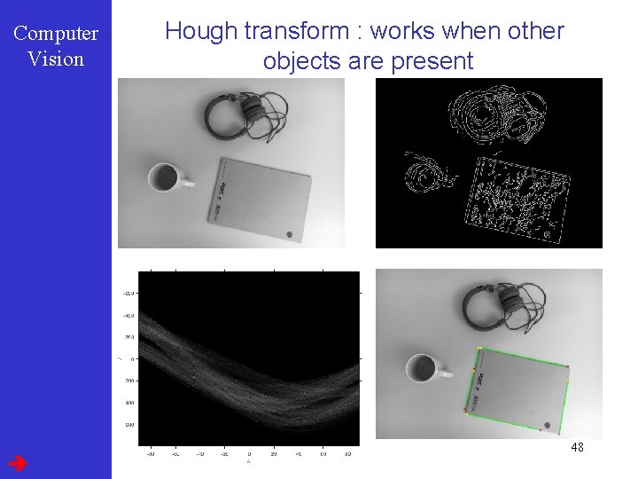
Computer Vision Hough transform : works when other objects are present 48

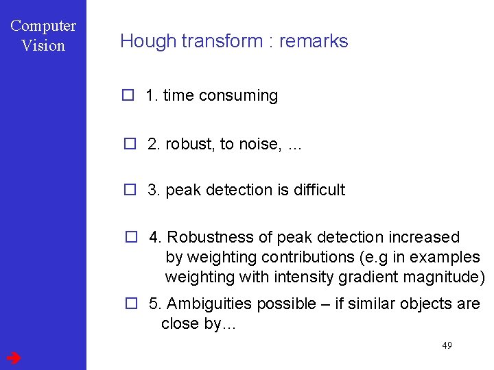
Computer Vision Hough transform : remarks o 1. time consuming o 2. robust, to noise, … o 3. peak detection is difficult o 4. Robustness of peak detection increased by weighting contributions (e. g in examples weighting with intensity gradient magnitude) o 5. Ambiguities possible – if similar objects are close by… 49

Computer Vision Segmentation : Outline l Thresholding l Edge based l Region based l Statistical Pattern Recognition based 50

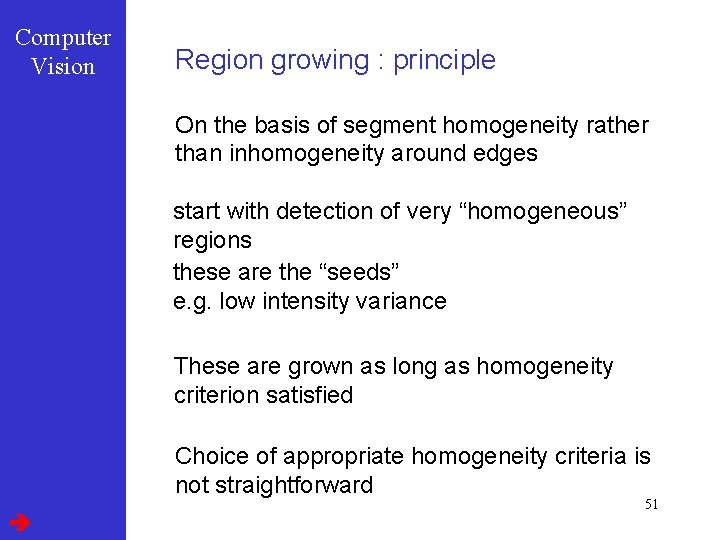
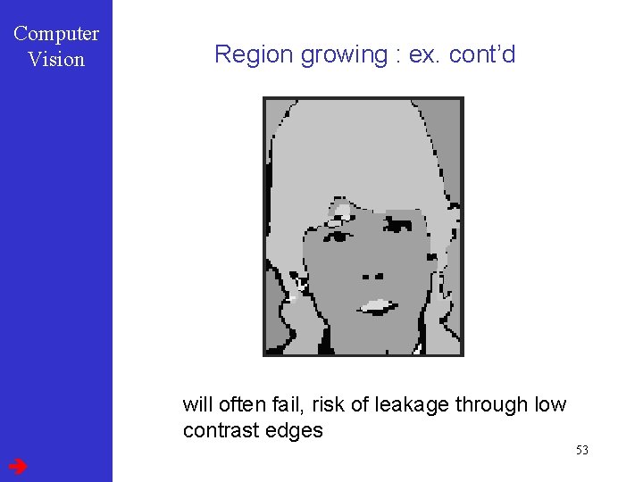
Computer Vision Region growing : principle On the basis of segment homogeneity rather than inhomogeneity around edges start with detection of very “homogeneous” regions these are the “seeds” e. g. low intensity variance These are grown as long as homogeneity criterion satisfied Choice of appropriate homogeneity criteria is not straightforward 51

Computer Vision Region growing : example Seeds of low intensity variance are grown, keeping intensity between two slowly floating thresholds and merging overlapping segments 52

Computer Vision Region growing : ex. cont’d will often fail, risk of leakage through low contrast edges 53

Computer Vision Region growing : remarks region growing pure is a one-way process : if seeds are wrong, errors cannot be corrected solution : split-and-merge procedures merges of similar regions splitting more difficult : many ways to do it splitting calls for special decompositions of segments, e. g. “quadtrees” Region and edge based methods can be combined: hybrid approaches 54

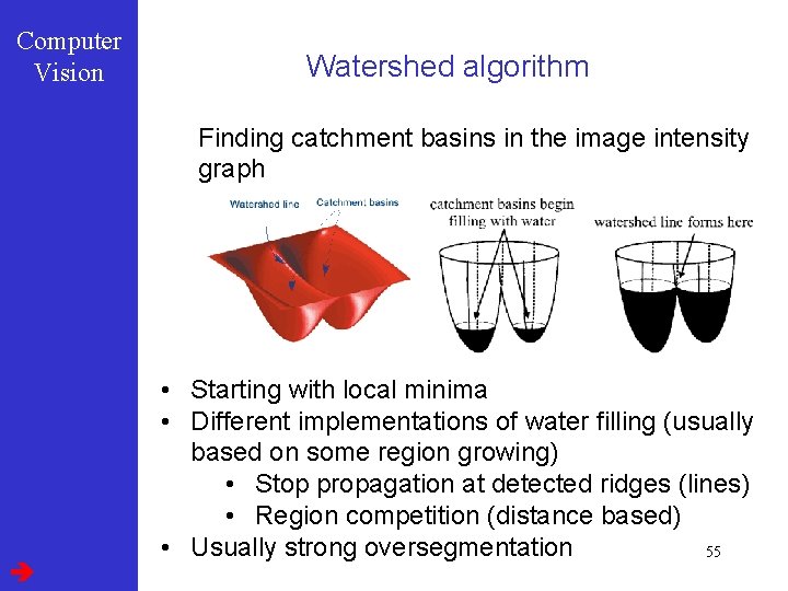
Computer Vision Watershed algorithm Finding catchment basins in the image intensity graph • Starting with local minima • Different implementations of water filling (usually based on some region growing) • Stop propagation at detected ridges (lines) • Region competition (distance based) • Usually strong oversegmentation 55

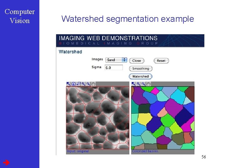
Computer Vision Watershed segmentation example 56

Computer Vision Segmentation : Outline l Thresholding l Edge based l Region based l Statistical Pattern Recognition based 57

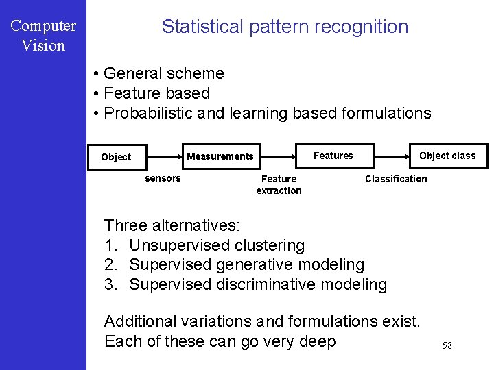
Statistical pattern recognition Computer Vision • General scheme • Feature based • Probabilistic and learning based formulations Features Measurements Object sensors Feature extraction Object class Classification Three alternatives: 1. Unsupervised clustering 2. Supervised generative modeling 3. Supervised discriminative modeling Additional variations and formulations exist. Each of these can go very deep 58

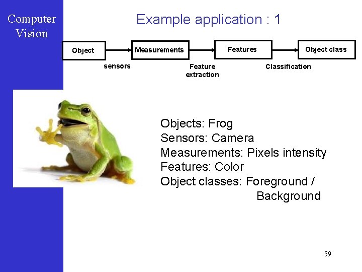
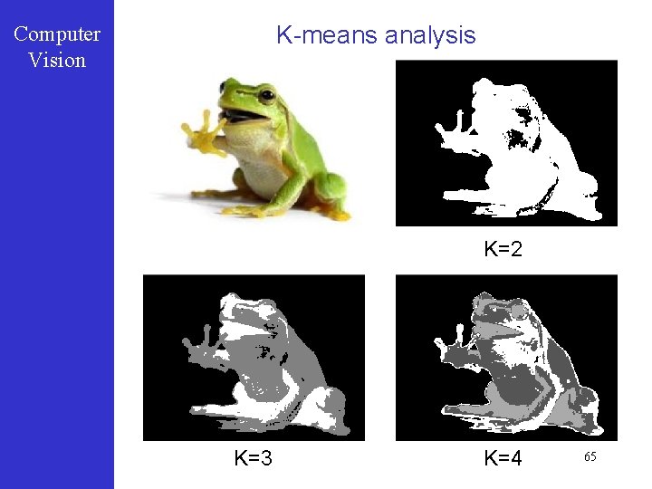
Example application : 1 Computer Vision Features Measurements Object sensors Feature extraction Object class Classification Objects: Frog Sensors: Camera Measurements: Pixels intensity Features: Color Object classes: Foreground / Background 59

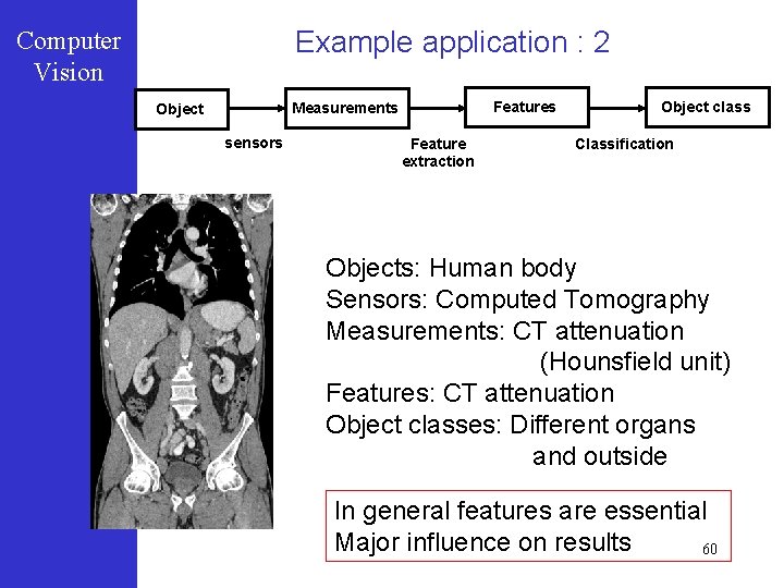
Example application : 2 Computer Vision Features Measurements Object sensors Feature extraction Object class Classification Objects: Human body Sensors: Computed Tomography Measurements: CT attenuation (Hounsfield unit) Features: CT attenuation Object classes: Different organs and outside In general features are essential Major influence on results 60

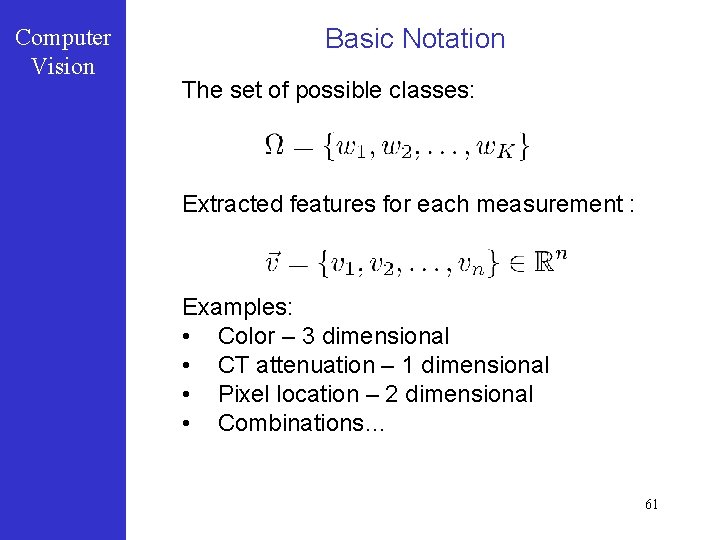
Computer Vision Basic Notation The set of possible classes: Extracted features for each measurement : Examples: • Color – 3 dimensional • CT attenuation – 1 dimensional • Pixel location – 2 dimensional • Combinations… 61

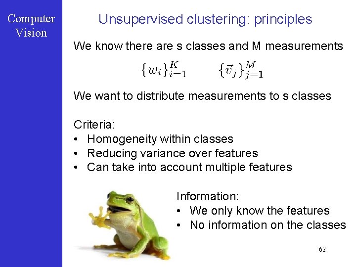
Computer Vision Unsupervised clustering: principles We know there are s classes and M measurements We want to distribute measurements to s classes Criteria: • Homogeneity within classes • Reducing variance over features • Can take into account multiple features Information: • We only know the features • No information on the classes 62

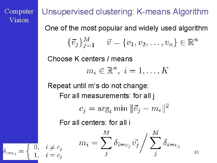
Computer Vision Unsupervised clustering: K-means Algorithm One of the most popular and widely used algorithm Choose K centers / means Repeat until m’s do not change: For all measurements: for all j For all centers: for all i 63

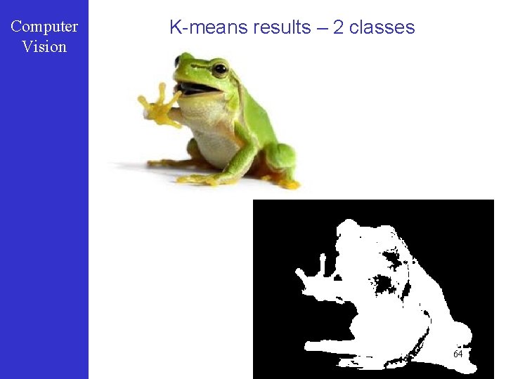
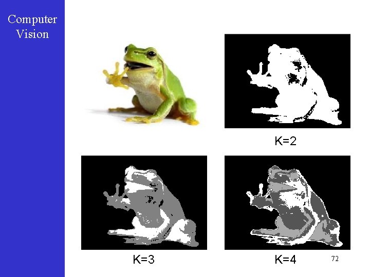
Computer Vision K-means results – 2 classes 64

K-means analysis Computer Vision K=2 K=3 K=4 65

Computer Vision K-means remarks Extremely easy to implement Useful initial analysis Choice of K has a major influence Methods exist to choose it automatically: Heuristic methods based on variance Non-parametric Bayesian Initialization is important K-means can get stuck in local minima Multiple initializations Multi-scale methods 66

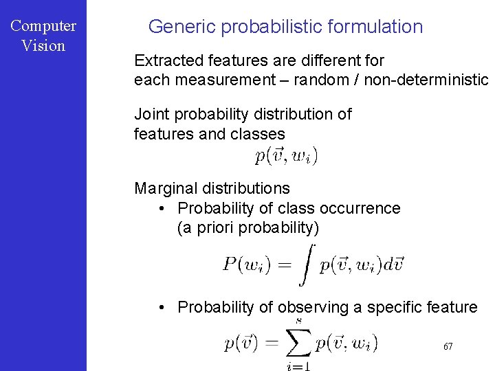
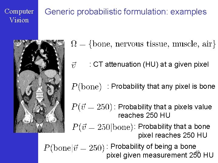
Computer Vision Generic probabilistic formulation Extracted features are different for each measurement – random / non-deterministic Joint probability distribution of features and classes Marginal distributions • Probability of class occurrence (a priori probability) • Probability of observing a specific feature 67

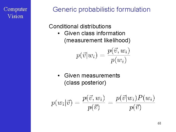
Computer Vision Generic probabilistic formulation Conditional distributions • Given class information (measurement likelihood) • Given measurements (class posterior) 68

Computer Vision Generic probabilistic formulation: examples : CT attenuation (HU) at a given pixel : Probability that any pixel is bone : Probability that a pixels value reaches 250 HU : Probability that a bone pixel reaches 250 HU : Probability of being a bone 69 pixel given measurement 250 HU

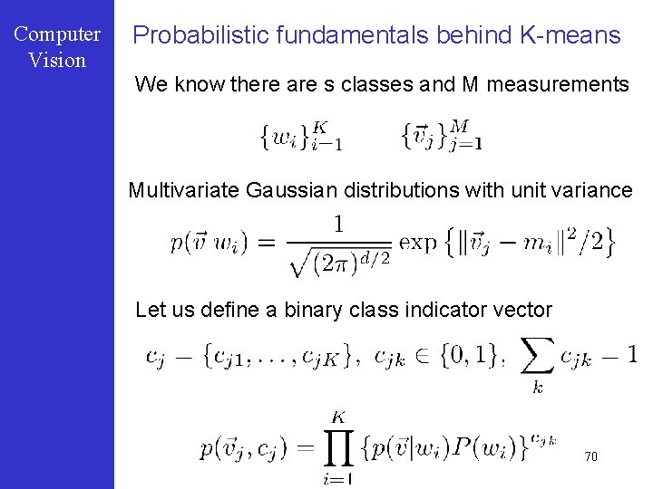
Computer Vision Probabilistic fundamentals behind K-means We know there are s classes and M measurements Multivariate Gaussian distributions with unit variance Let us define a binary class indicator vector 70

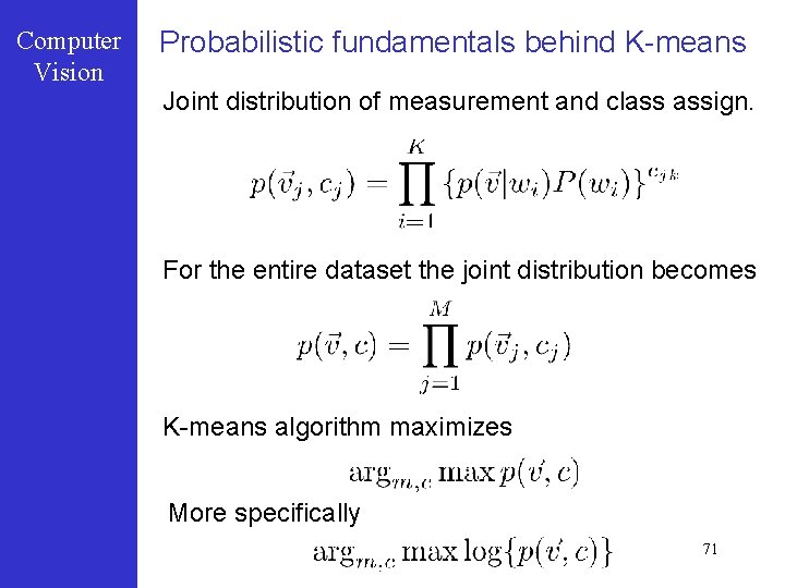
Computer Vision Probabilistic fundamentals behind K-means Joint distribution of measurement and class assign. For the entire dataset the joint distribution becomes K-means algorithm maximizes More specifically 71

Computer Vision K=2 K=3 K=4 72

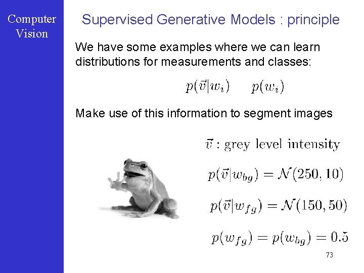
Computer Vision Supervised Generative Models : principle We have some examples where we can learn distributions for measurements and classes: Make use of this information to segment images 73

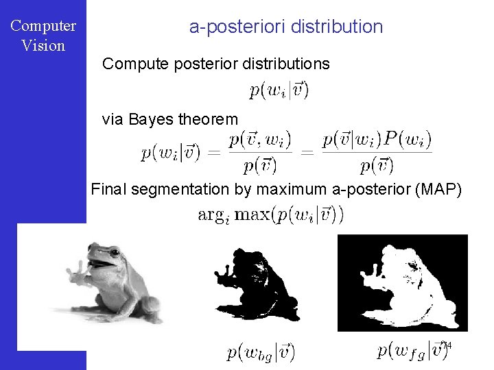
Computer Vision a-posteriori distribution Compute posterior distributions via Bayes theorem Final segmentation by maximum a-posterior (MAP) 74

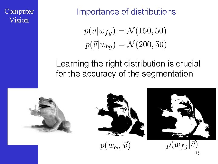
Computer Vision Importance of distributions Learning the right distribution is crucial for the accuracy of the segmentation 75

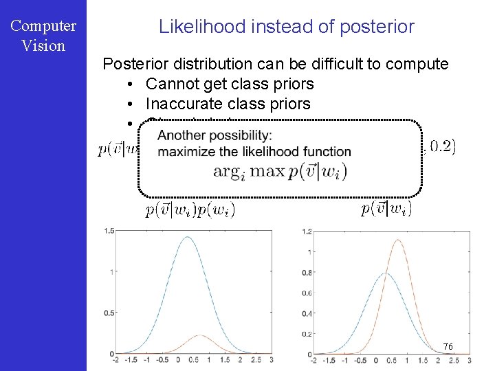
Computer Vision Likelihood instead of posterior Posterior distribution can be difficult to compute • Cannot get class priors • Inaccurate class priors • Class imbalance 76

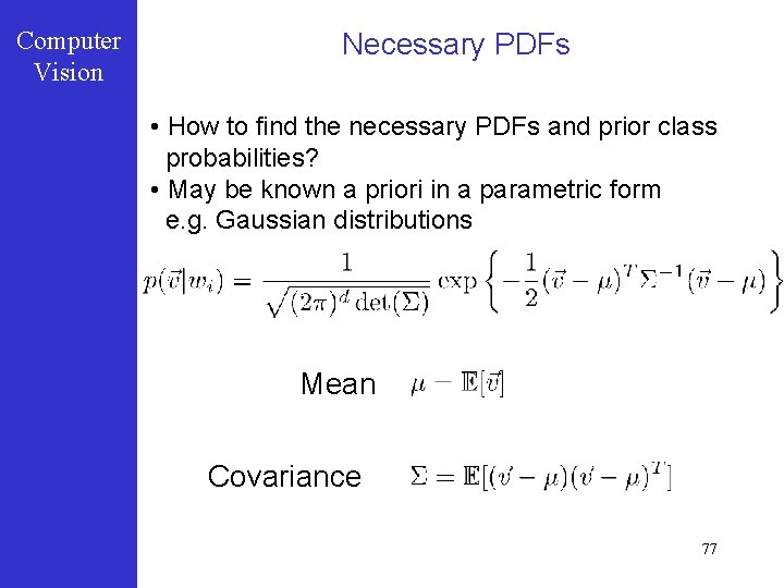
Computer Vision Necessary PDFs • How to find the necessary PDFs and prior class probabilities? • May be known a priori in a parametric form e. g. Gaussian distributions Mean Covariance 77

Computer Vision Outline • Supervised generative learning: From individual pixels to combinations Markov Random Fields Gibbs sampling Graph-cuts • Supervised discriminative learning for segmentation KNN Random Forests 78

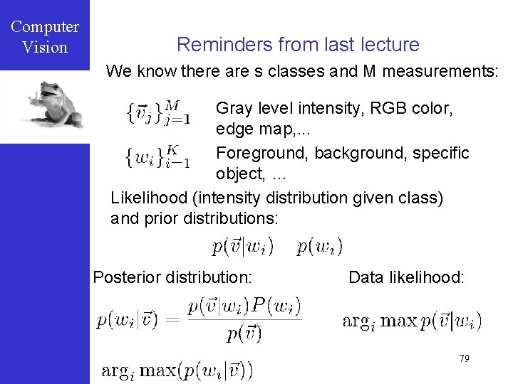
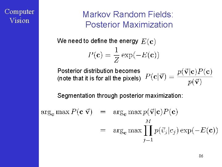
Computer Vision Reminders from last lecture We know there are s classes and M measurements: Gray level intensity, RGB color, edge map, . . . Foreground, background, specific object, … Likelihood (intensity distribution given class) and prior distributions: Posterior distribution: Data likelihood: 79

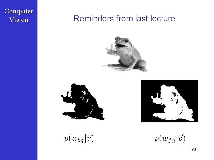
Computer Vision Reminders from last lecture 80

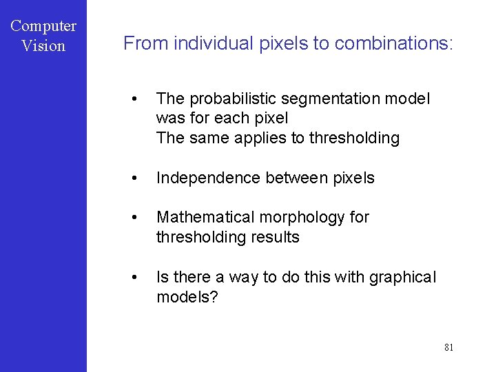
Computer Vision From individual pixels to combinations: • The probabilistic segmentation model was for each pixel The same applies to thresholding • Independence between pixels • Mathematical morphology for thresholding results • Is there a way to do this with graphical models? 81

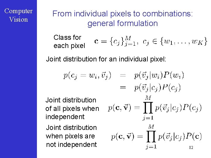
Computer Vision From individual pixels to combinations: general formulation Class for each pixel Joint distribution for an individual pixel: Joint distribution of all pixels when independent Joint distribution when pixels are not independent 82

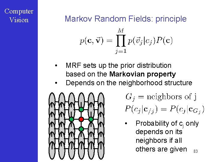
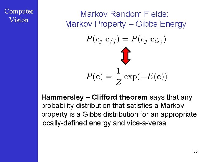
Computer Vision Markov Random Fields: principle • • MRF sets up the prior distribution based on the Markovian property Depends on the neighborhood structure • Probability of cj only depends on its neighbors if all others are given 83

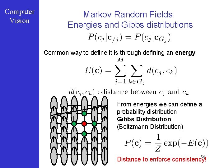
Computer Vision Markov Random Fields: Energies and Gibbs distributions Common way to define it is through defining an energy From energies we can define a probability distribution Gibbs Distribution (Boltzmann Distribution) 84 Distance to enforce consistency!

Computer Vision Markov Random Fields: Markov Property – Gibbs Energy Hammersley – Clifford theorem says that any probability distribution that satisfies a Markov property is a Gibbs distribution for an appropriate locally-defined energy and vice-a-versa. 85

Computer Vision Markov Random Fields: Posterior Maximization We need to define the energy Posterior distribution becomes (note that it is for all the pixels) Segmentation through posterior maximization: 86

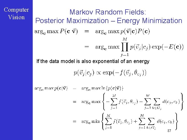
Computer Vision Markov Random Fields: Posterior Maximization – Energy Minimization If the data model is also exponential of an energy 87

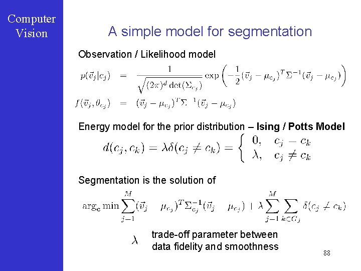
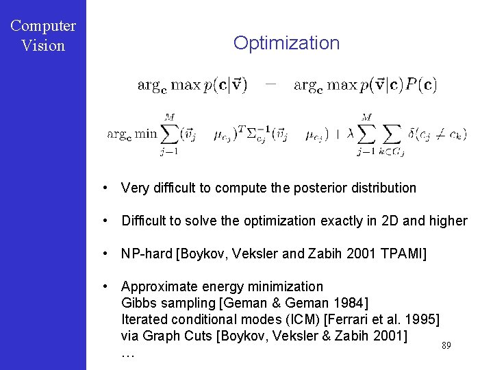
Computer Vision A simple model for segmentation Observation / Likelihood model Energy model for the prior distribution – Ising / Potts Model Segmentation is the solution of trade-off parameter between data fidelity and smoothness 88

Computer Vision Optimization • Very difficult to compute the posterior distribution • Difficult to solve the optimization exactly in 2 D and higher • NP-hard [Boykov, Veksler and Zabih 2001 TPAMI] • Approximate energy minimization Gibbs sampling [Geman & Geman 1984] Iterated conditional modes (ICM) [Ferrari et al. 1995] via Graph Cuts [Boykov, Veksler & Zabih 2001] 89 …

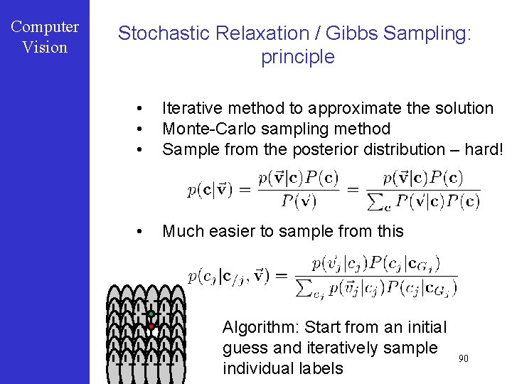
Computer Vision Stochastic Relaxation / Gibbs Sampling: principle • • • Iterative method to approximate the solution Monte-Carlo sampling method Sample from the posterior distribution – hard! • Much easier to sample from this Algorithm: Start from an initial guess and iteratively sample individual labels 90

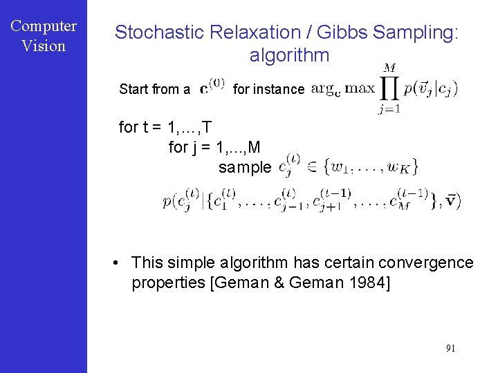
Computer Vision Stochastic Relaxation / Gibbs Sampling: algorithm Start from a for instance for t = 1, …, T for j = 1, . . . , M sample • This simple algorithm has certain convergence properties [Geman & Geman 1984] 91

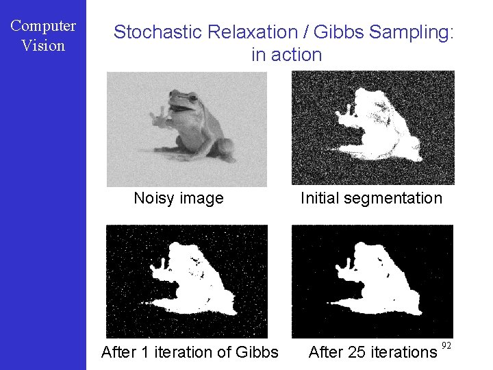
Computer Vision Stochastic Relaxation / Gibbs Sampling: in action Noisy image After 1 iteration of Gibbs Initial segmentation After 25 iterations 92

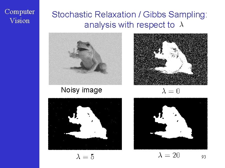
Computer Vision Stochastic Relaxation / Gibbs Sampling: analysis with respect to Noisy image 93

Computer Vision Stochastic Relaxation / Gibbs Sampling: remarks • Very simplementation and effective • Solution depends on the parameter • Solution depends on initial condition • May not converge to a pleasing result • Not very efficient – convergence is slow • Stochastic in nature 94

Computer Vision Remarks on Generative Supervised Models • • Mathematically sound Flexible and generic Model specifications can change Can be extended to various features Wealth of research Links to Bayesian methods Features are very important Optimization and inference can be hard For high dimensional features estimation of distributions can be problematic Latent variables / factors 95

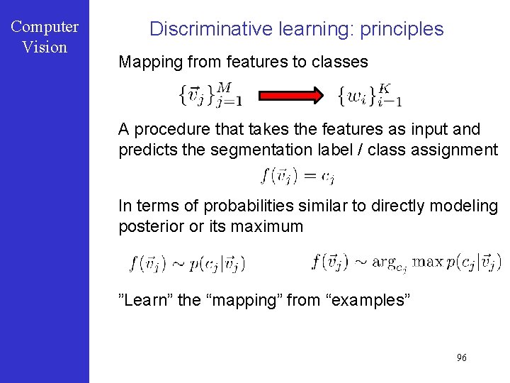
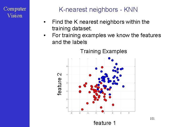
Computer Vision Discriminative learning: principles Mapping from features to classes A procedure that takes the features as input and predicts the segmentation label / class assignment In terms of probabilities similar to directly modeling posterior or its maximum ”Learn” the “mapping” from “examples” 96

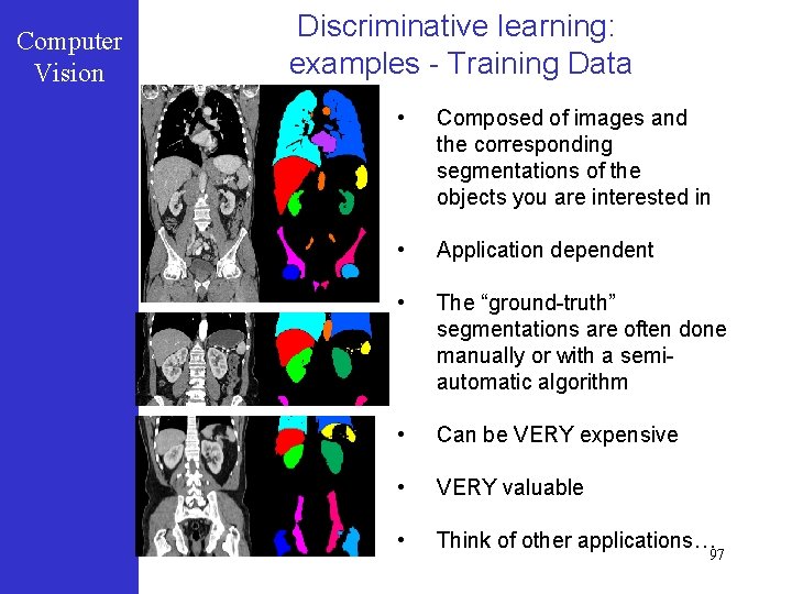
Computer Vision Discriminative learning: examples - Training Data • Composed of images and the corresponding segmentations of the objects you are interested in • Application dependent • The “ground-truth” segmentations are often done manually or with a semiautomatic algorithm • Can be VERY expensive • VERY valuable • Think of other applications… 97

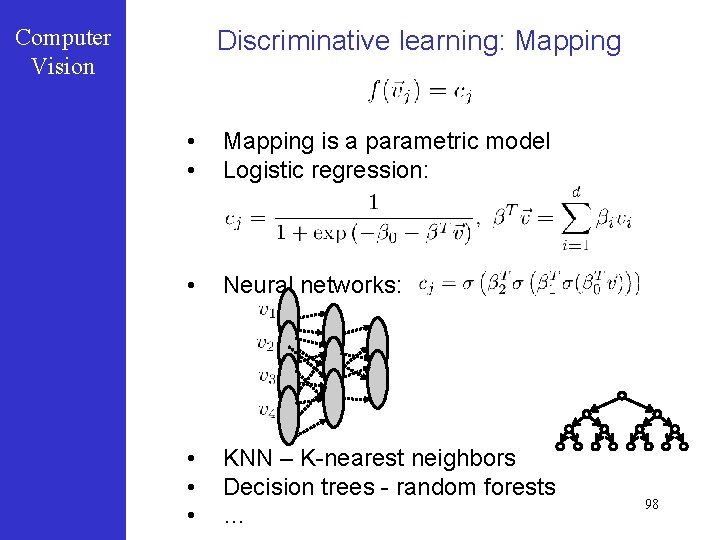
Computer Vision Discriminative learning: Mapping • • Mapping is a parametric model Logistic regression: • Neural networks: • • • KNN – K-nearest neighbors Decision trees - random forests … 98

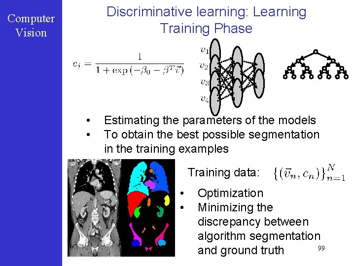
Discriminative learning: Learning Training Phase Computer Vision • • Estimating the parameters of the models To obtain the best possible segmentation in the training examples Training data: • • Optimization Minimizing the discrepancy between algorithm segmentation 99 and ground truth

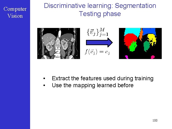
Computer Vision Discriminative learning: Segmentation Testing phase • • Extract the features used during training Use the mapping learned before 100

K-nearest neighbors - KNN • • Find the K nearest neighbors within the training dataset. For training examples we know the features and the labels Training Examples feature 2 Computer Vision feature 1 101

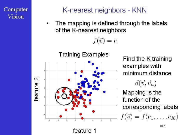
Computer Vision K-nearest neighbors - KNN • The mapping is defined through the labels of the K-nearest neighbors feature 2 Training Examples Find the K training examples with minimum distance Mapping is the function of the corresponding labels feature 1 102

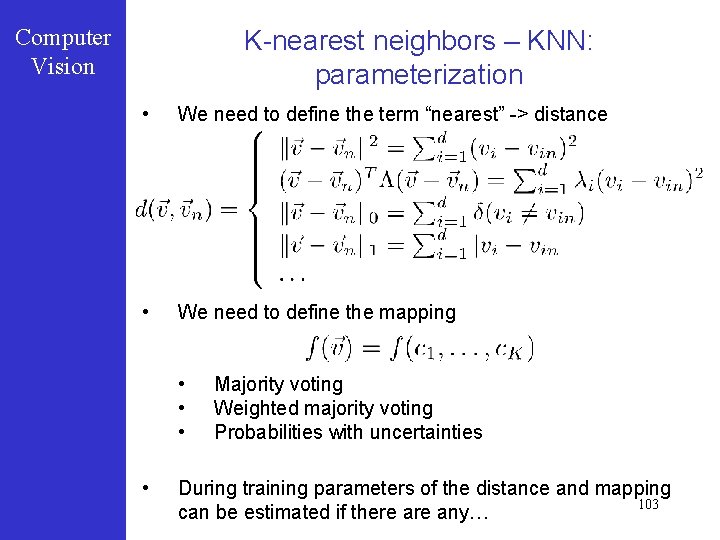
Computer Vision K-nearest neighbors – KNN: parameterization • We need to define the term “nearest” -> distance • We need to define the mapping • • Majority voting Weighted majority voting Probabilities with uncertainties During training parameters of the distance and mapping 103 can be estimated if there any…

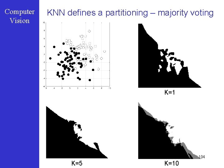
Computer Vision KNN defines a partitioning – majority voting K=1 104 K=5 K=10

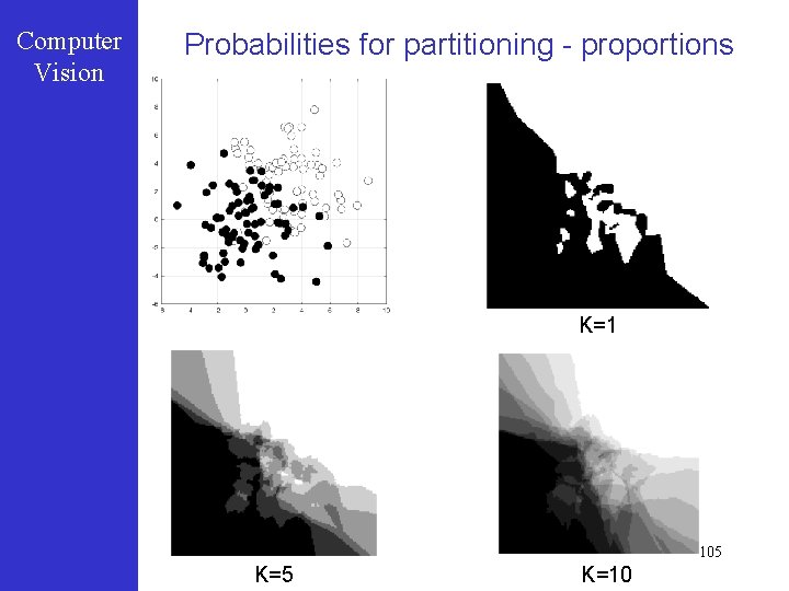
Computer Vision Probabilities for partitioning - proportions K=1 105 K=10

Computer Vision Remarks on KNN • • Very simple to implement Very simple to understand Efficient implementations possible approximate nearest neighbors, … Distance definition is flexible Highly depends on the definitions and K Need to keep the entire data in memory for distance computations For high dimensional problems (with high d) need a LOT of training samples for accuracy Other algorithms for high dimensional: Random forests Neural networks (deep learning) 106 …

Computer Vision -Optional Part- 107

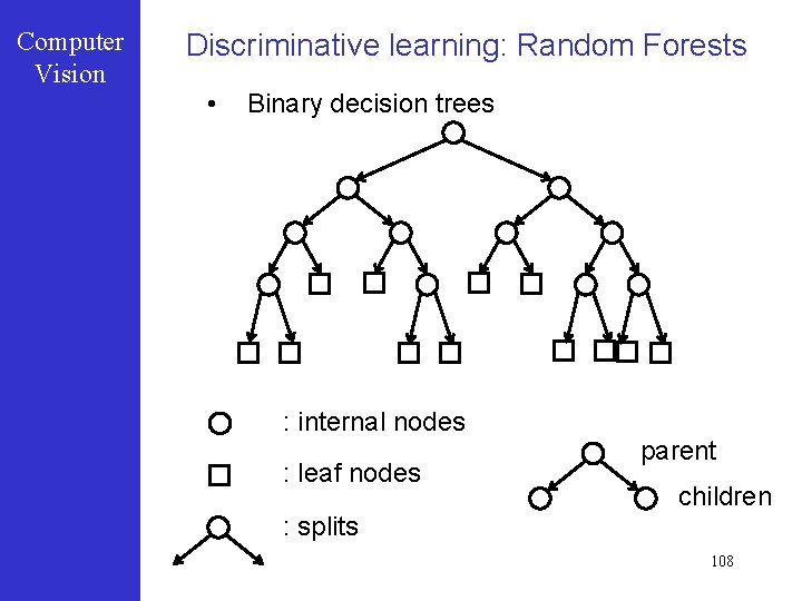
Computer Vision Discriminative learning: Random Forests • Binary decision trees : internal nodes : leaf nodes parent children : splits 108

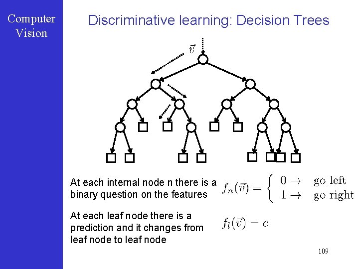
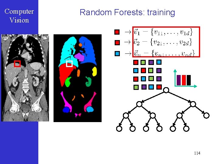
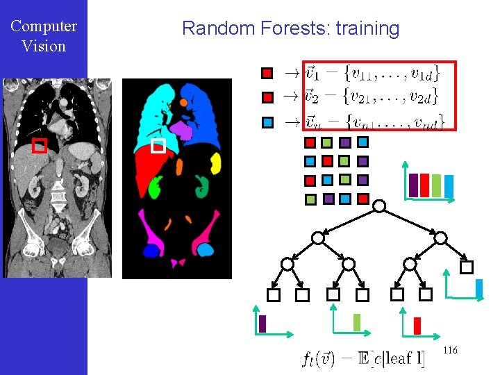
Computer Vision Discriminative learning: Decision Trees At each internal node n there is a binary question on the features At each leaf node there is a prediction and it changes from leaf node to leaf node 109

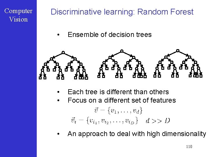
Computer Vision Discriminative learning: Random Forest • Ensemble of decision trees • • Each tree is different than others Focus on a different set of features • An approach to deal with high dimensionality 110

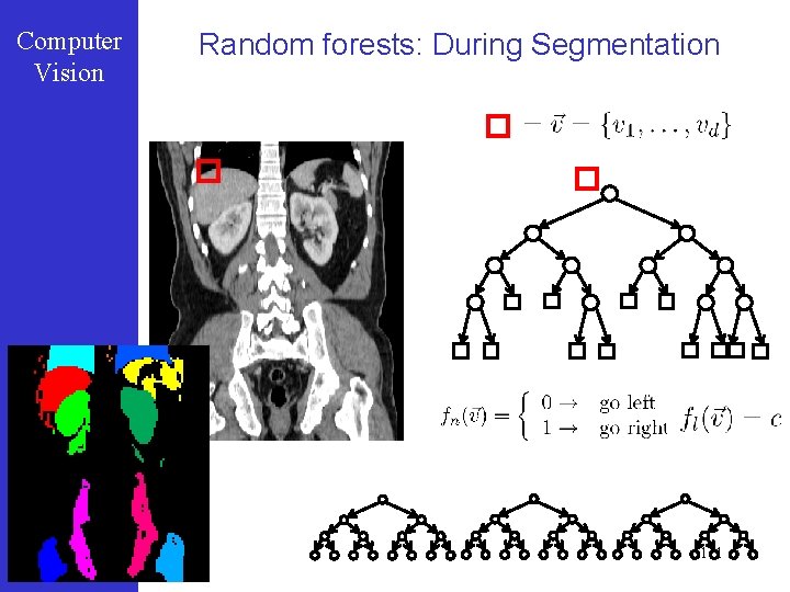
Computer Vision Random forests: During Segmentation 111

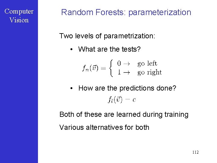
Computer Vision Random Forests: parameterization Two levels of parametrization: • What are the tests? • How are the predictions done? Both of these are learned during training Various alternatives for both 112

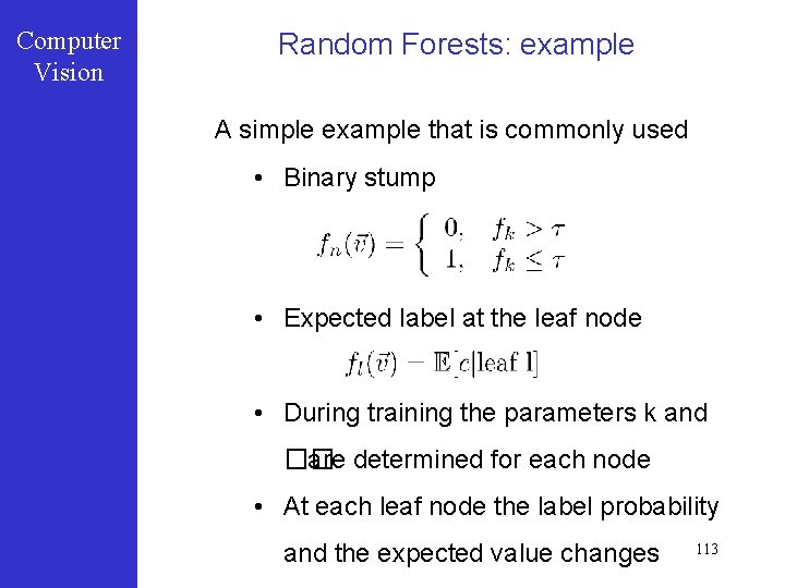
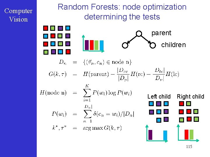
Computer Vision Random Forests: example A simple example that is commonly used • Binary stump • Expected label at the leaf node • During training the parameters k and �� are determined for each node • At each leaf node the label probability and the expected value changes 113

Computer Vision Random Forests: training 114

Computer Vision Random Forests: node optimization determining the tests parent children Left child Right child 115

Computer Vision Random Forests: training 116

Computer Vision Random Forests: remarks • Easy to implement • VERY efficient • Technology behind Kinect (earlier version) • Lots of parametric choices • Needs large number of data • Training can take time 117