Computer Vision What is Computer Vision Input images

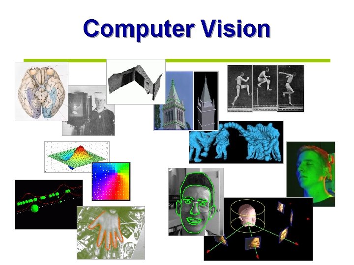
Computer Vision

What is Computer Vision? • Input: images or video • Output: description of the world • But also: measuring, classifying, interpreting visual information

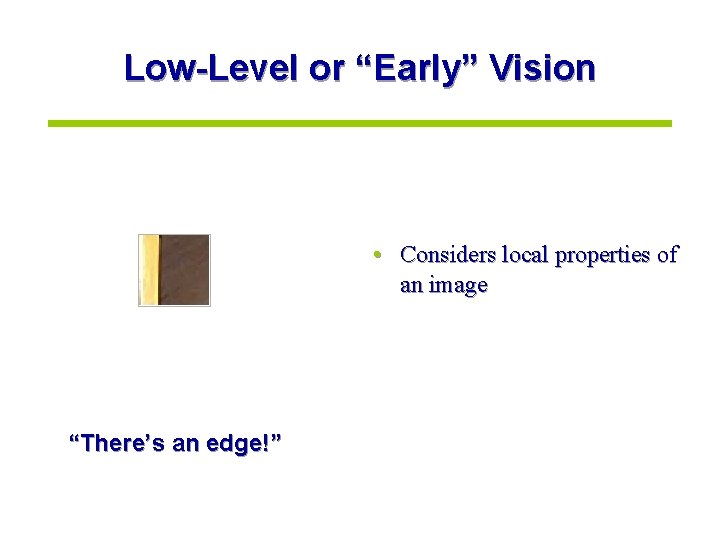
Low-Level or “Early” Vision • Considers local properties of an image “There’s an edge!”

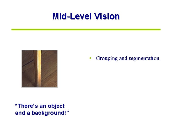
Mid-Level Vision • Grouping and segmentation “There’s an object and a background!”

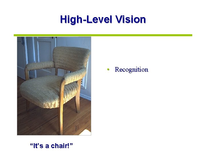
High-Level Vision • Recognition “It’s a chair!”

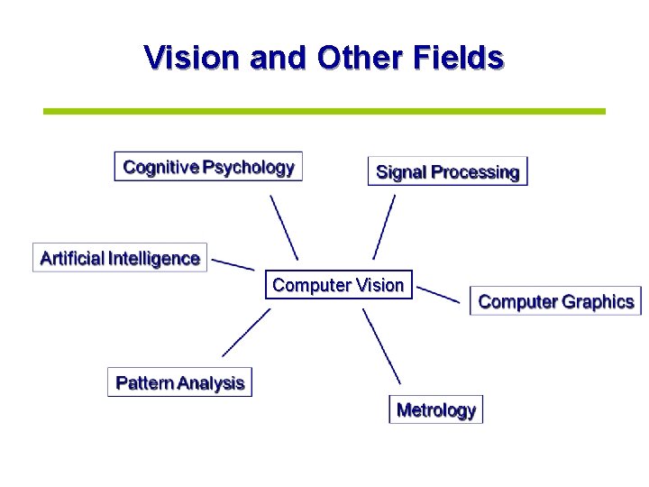
Vision and Other Fields Computer Vision

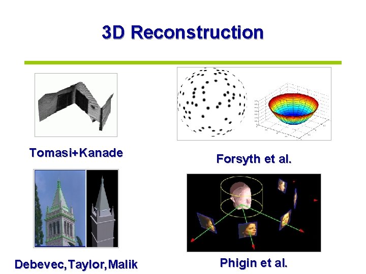
3 D Reconstruction Tomasi+Kanade Forsyth et al. Debevec, Taylor, Malik Phigin et al.

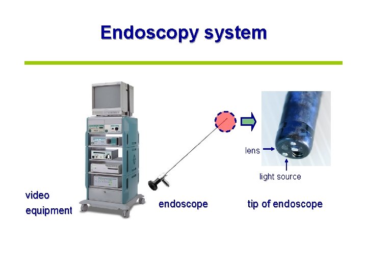
Endoscopy system lens light source video equipment endoscope tip of endoscope

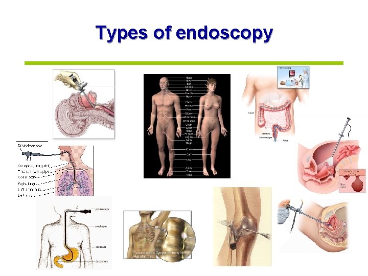
Types of endoscopy

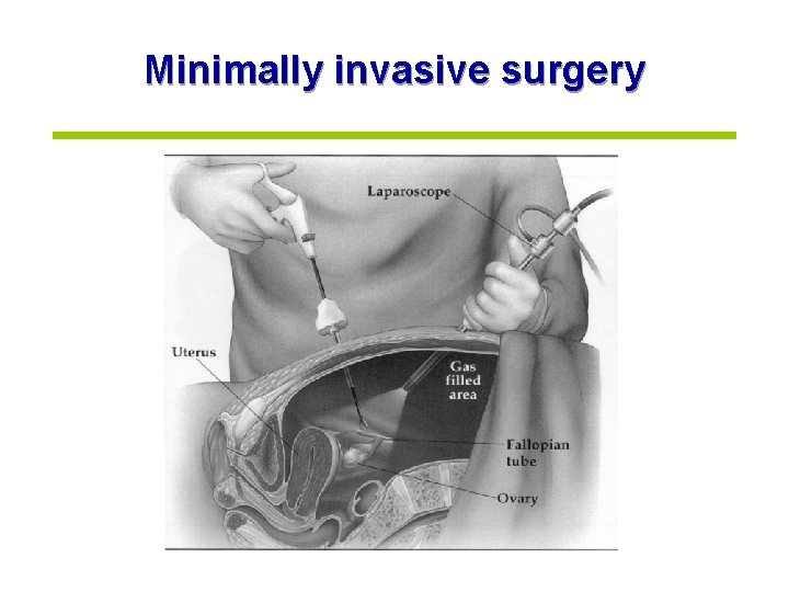
Minimally invasive surgery

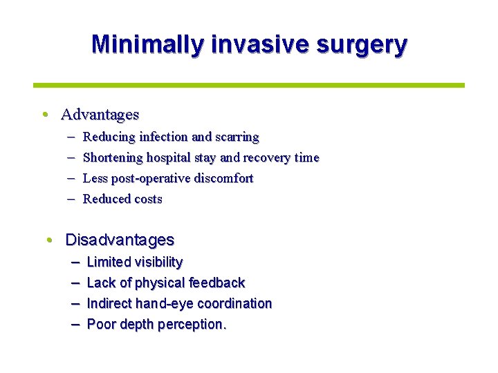
Minimally invasive surgery • Advantages – – Reducing infection and scarring Shortening hospital stay and recovery time Less post-operative discomfort Reduced costs • Disadvantages – – Limited visibility Lack of physical feedback Indirect hand-eye coordination Poor depth perception.

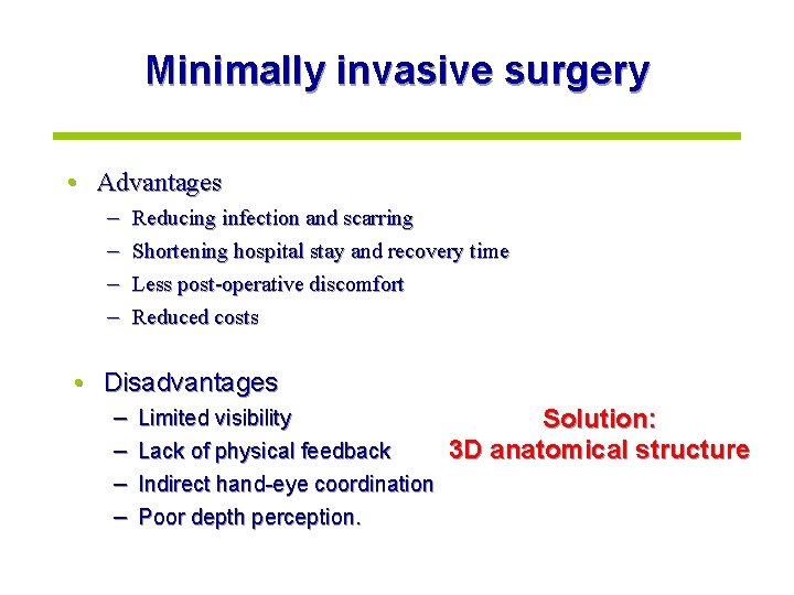
Minimally invasive surgery • Advantages – – Reducing infection and scarring Shortening hospital stay and recovery time Less post-operative discomfort Reduced costs • Disadvantages – – Limited visibility Lack of physical feedback Indirect hand-eye coordination Poor depth perception. Solution: 3 D anatomical structure

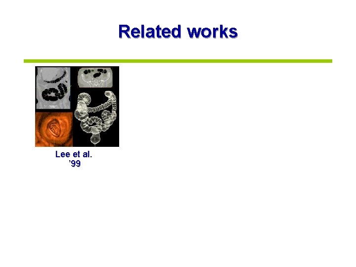
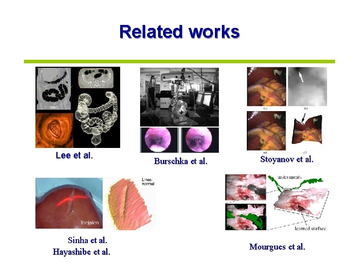
Related works Lee et al. ’ 99

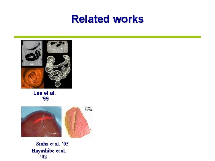
Related works Lee et al. ’ 99 Sinha et al. ’ 05 Hayashibe et al. ’ 02

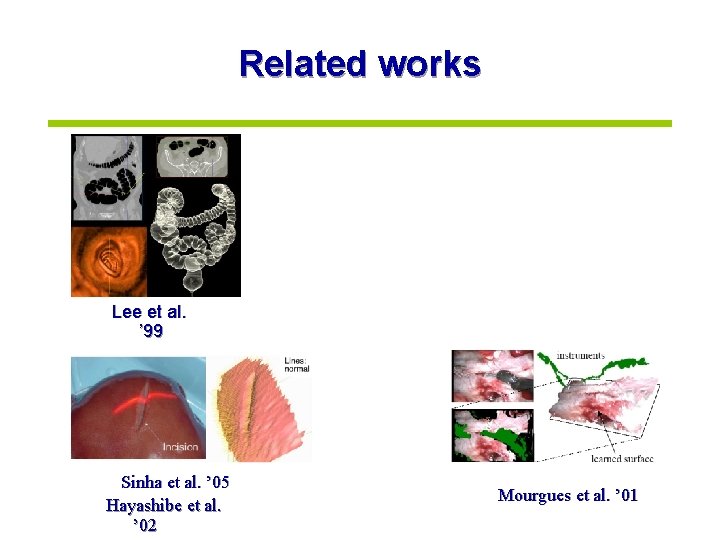
Related works Lee et al. ’ 99 Sinha et al. ’ 05 Hayashibe et al. ’ 02 Mourgues et al. ’ 01

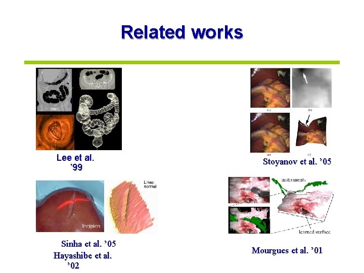
Related works Lee et al. ’ 99 Sinha et al. ’ 05 Hayashibe et al. ’ 02 Stoyanov et al. ’ 05 Mourgues et al. ’ 01

Related works Lee et al. Sinha et al. Hayashibe et al. Burschka et al. Stoyanov et al. Mourgues et al.

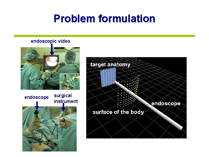
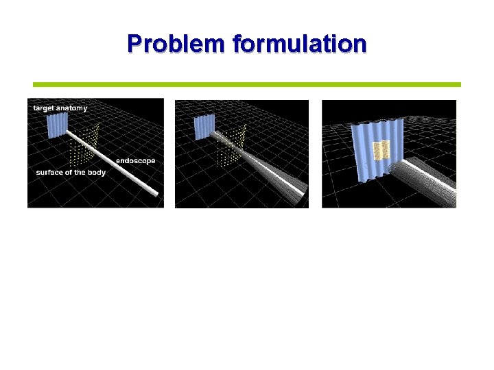
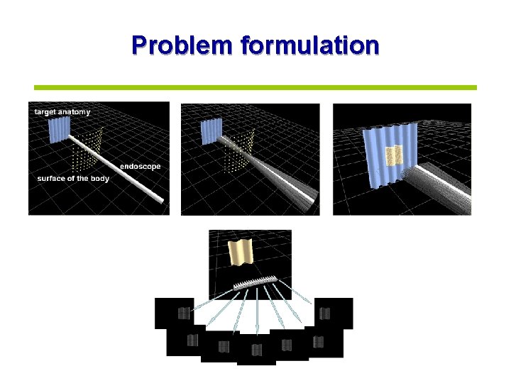
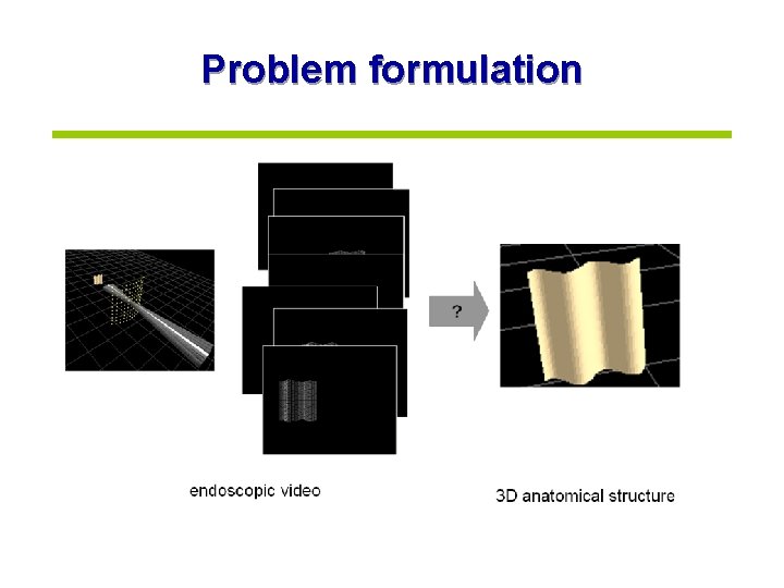
Problem formulation endoscopic video endoscope surgical instrument

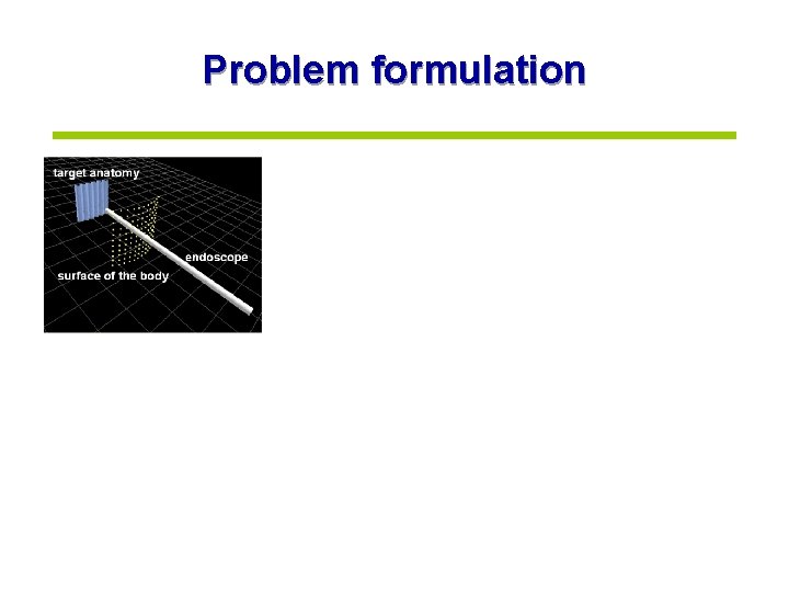
Problem formulation

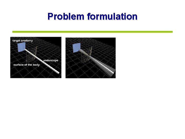
Problem formulation

Problem formulation

Problem formulation

Problem formulation

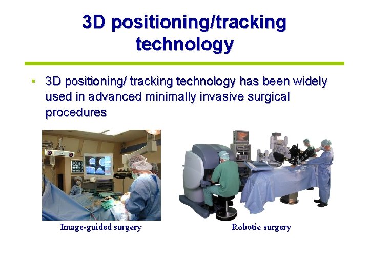
3 D positioning/tracking technology • 3 D positioning/ tracking technology has been widely used in advanced minimally invasive surgical procedures Image-guided surgery Robotic surgery

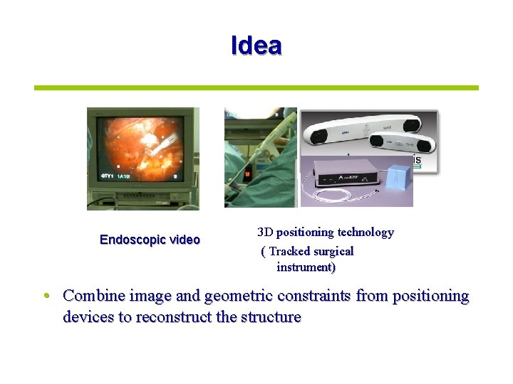
Idea Endoscopic video 3 D positioning technology ( Tracked surgical instrument) • Combine image and geometric constraints from positioning devices to reconstruct the structure

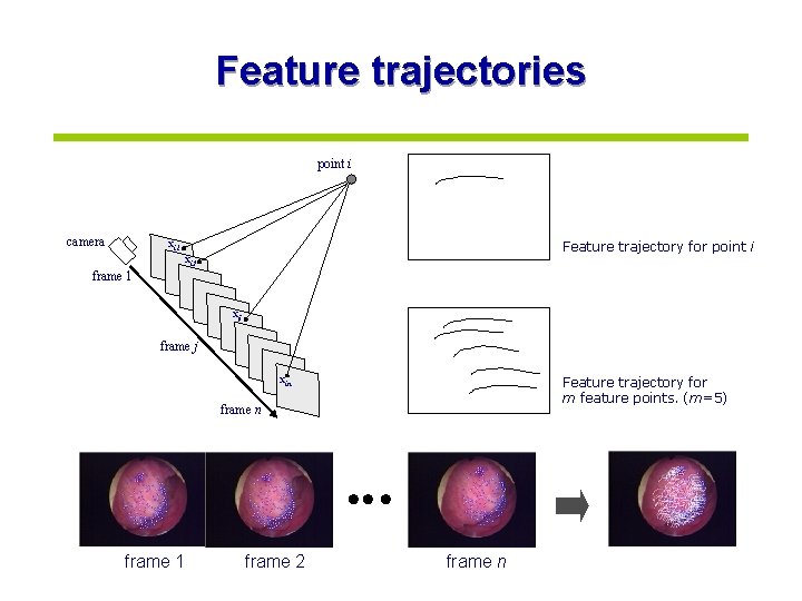
Feature trajectories point i camera xi 1 Feature trajectory for point i xi 2 frame 1 xij frame j xin Feature trajectory for m feature points. (m=5) frame n frame 1 frame 2 frame n

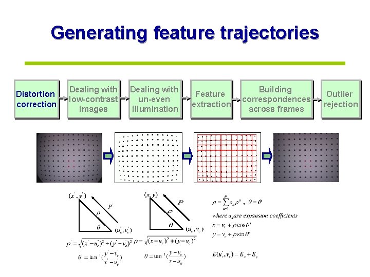
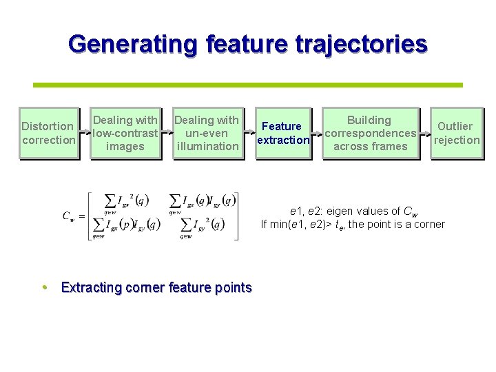
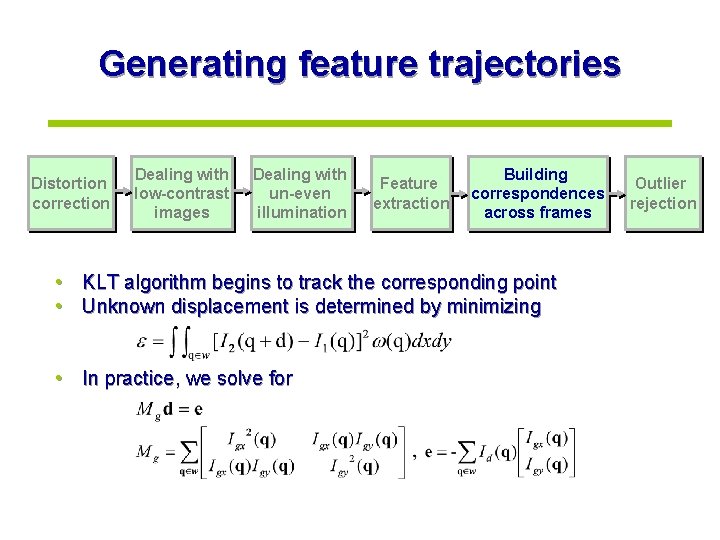
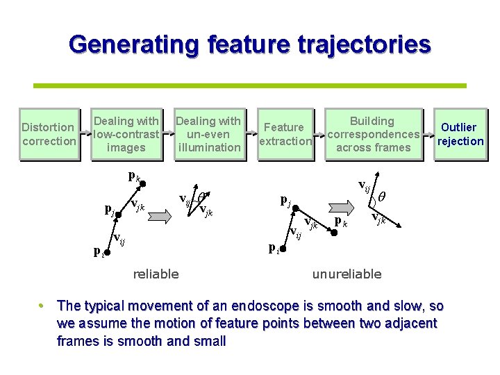
Generating feature trajectories Distortion correction Dealing with low-contrast images Dealing with un-even illumination Feature extraction Building correspondences across frames Outlier rejection

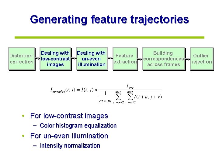
Generating feature trajectories Distortion correction Dealing with low-contrast images Dealing with un-even illumination Feature extraction • For low-contrast images – Color histogram equalization • For un-even illumination – Intensity normalization Building correspondences across frames Outlier rejection

Generating feature trajectories Distortion correction Dealing with low-contrast images Dealing with un-even illumination Feature extraction Building correspondences across frames Outlier rejection e 1, e 2: eigen values of Cw If min(e 1, e 2)> te, the point is a corner • Extracting corner feature points

Generating feature trajectories Distortion correction Dealing with low-contrast images Dealing with un-even illumination Feature extraction Building correspondences across frames • KLT algorithm begins to track the corresponding point • Unknown displacement is determined by minimizing • In practice, we solve for Outlier rejection

Generating feature trajectories Distortion correction Dealing with low-contrast images Dealing with un-even illumination Building correspondences across frames Feature extraction pk pj pi vjk vij vjk pj pi reliable vij vjk pk Outlier rejection vjk unureliable • The typical movement of an endoscope is smooth and slow, so we assume the motion of feature points between two adjacent frames is smooth and small

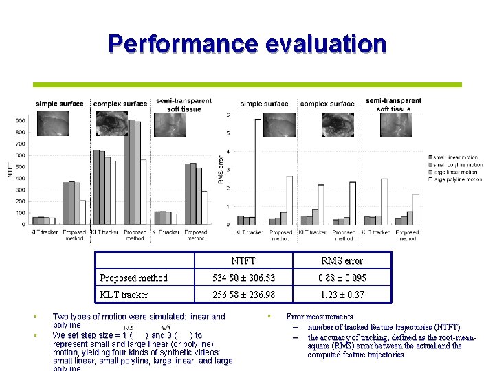
Performance evaluation • • NTFT RMS error Proposed method 534. 50 306. 53 0. 88 0. 095 KLT tracker 256. 58 236. 98 1. 23 0. 37 Two types of motion were simulated: linear and polyline We set step size = 1 ( ) and 3 ( ) to represent small and large linear (or polyline) motion, yielding four kinds of synthetic videos: small linear, small polyline, large linear, and large • Error measurements – number of tracked feature trajectories (NTFT) – the accuracy of tracking, defined as the root-meansquare (RMS) error between the actual and the computed feature trajectories

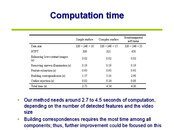
Computation time Simple surface Complex surface Semitransparent soft tissue 320 × 240 × 18 320 × 240 × 15 320 × 240 × 33 NTFT 308 821 458 Enhancing low-contrast images (s) 0. 02 Removing uneven illumination (s) 0. 19 Feature extraction (s) 0. 93 Building correspondences (s) 1. 57 3. 16 2. 98 Outlier rejection (s) 0. 02 0. 24 0. 08 Total time (s) 2. 73 4. 54 4. 20 Data size • Our method needs around 2. 7 to 4. 5 seconds of computation, depending on the number of detected features and the video size • Building correspondences requires the most time among all components; thus, further improvement could be focused on this

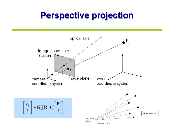
Perspective projection

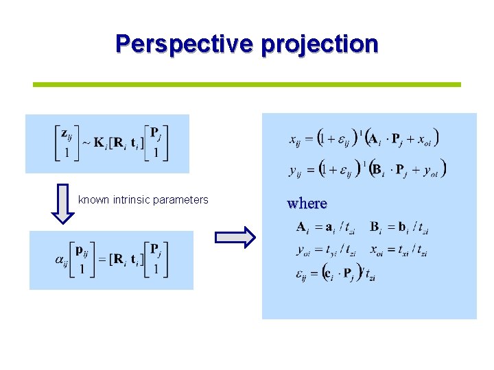
Perspective projection known intrinsic parameters where

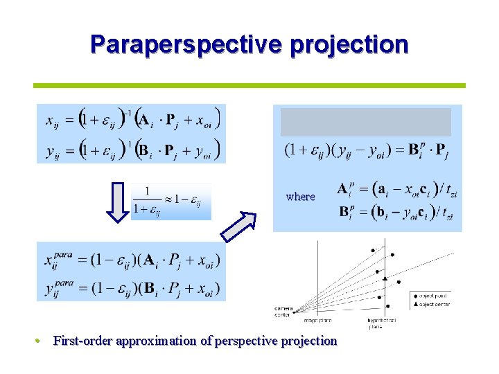
Paraperspective projection where • First-order approximation of perspective projection

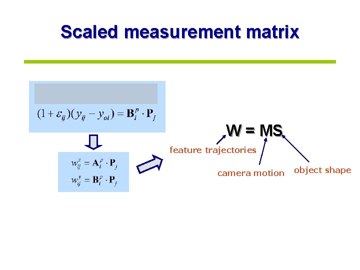
Scaled measurement matrix W = MS feature trajectories camera motion object shape

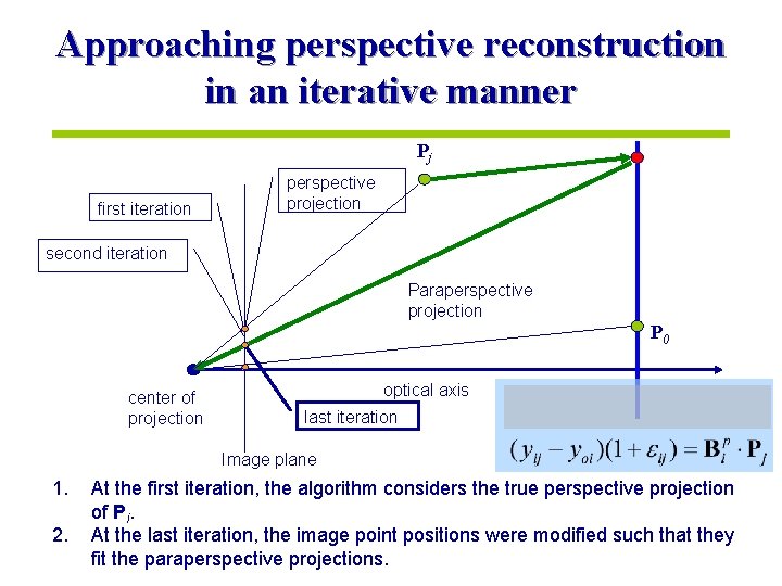
Approaching perspective reconstruction in an iterative manner Pj first iteration perspective projection second iteration Paraperspective projection P 0 center of projection optical axis last iteration Image plane 1. 2. At the first iteration, the algorithm considers the true perspective projection of Pi. At the last iteration, the image point positions were modified such that they fit the paraperspective projections.

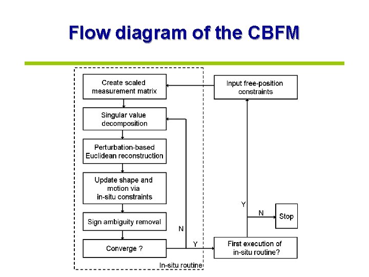
Flow diagram of the CBFM

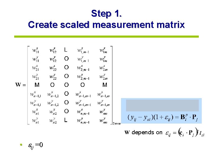
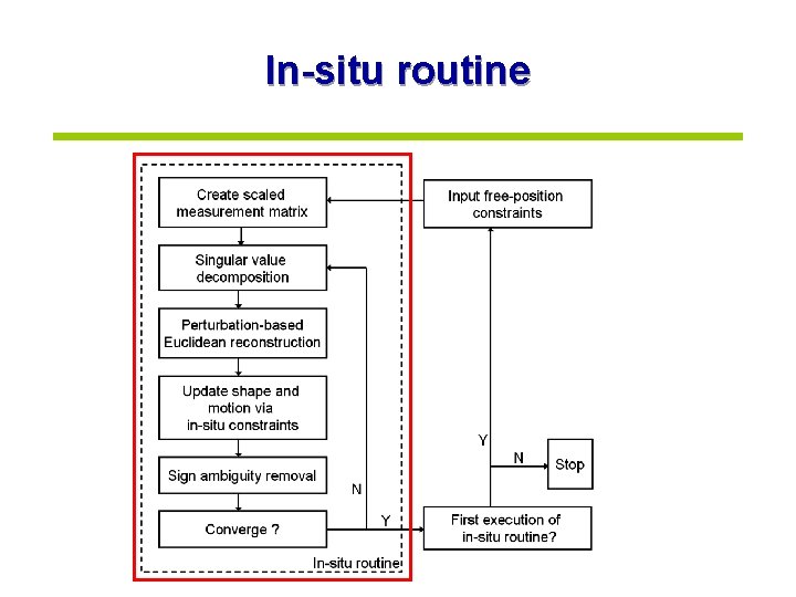
Step 1. Create scaled measurement matrix W depends on • ij =0

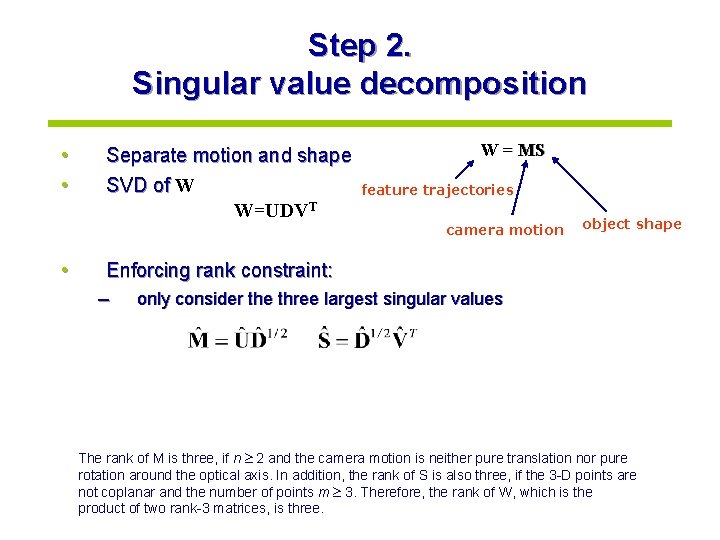
Step 2. Singular value decomposition • • • Separate motion and shape SVD of W W=UDVT W = MS feature trajectories camera motion object shape Enforcing rank constraint: – only consider the three largest singular values The rank of M is three, if n 2 and the camera motion is neither pure translation nor pure rotation around the optical axis. In addition, the rank of S is also three, if the 3 -D points are not coplanar and the number of points m 3. Therefore, the rank of W, which is the product of two rank-3 matrices, is three.

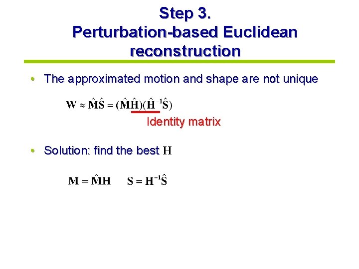
Step 3. Perturbation-based Euclidean reconstruction • The approximated motion and shape are not unique Identity matrix • Solution: find the best H

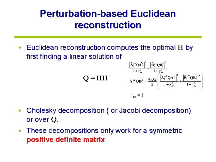
Perturbation-based Euclidean reconstruction • Euclidean reconstruction computes the optimal H by first finding a linear solution of Q = HHT • Cholesky decomposition ( or Jacobi decomposition) or over Q. • These decompositions only work for a symmetric positive definite matrix

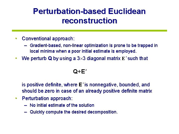
Perturbation-based Euclidean reconstruction • Conventional approach: – Gradient-based, non-linear optimization is prone to be trapped in local minima when a poor initial estimate is employed. • We perturb Q by using a 3 3 diagonal matrix E' such that Q+E' is positive definite, where E' is nonnegative, bounded, and should be zero in case of an already positive definite matrix • Perturbation approach: – No initial estimate of the solution – Quickly compute the desired decomposition.

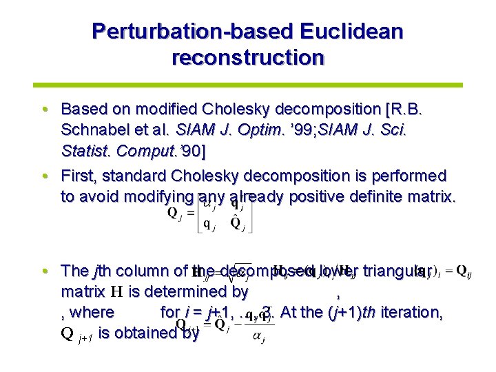
Perturbation-based Euclidean reconstruction • Based on modified Cholesky decomposition [R. B. Schnabel et al. SIAM J. Optim. ’ 99; SIAM J. Sci. Statist. Comput. ’ 90] • First, standard Cholesky decomposition is performed to avoid modifying any already positive definite matrix. • The jth column of the decomposed lower triangular matrix H is determined by , , where for i = j+1, . . . , 3. At the (j+1)th iteration, Q j+1 is obtained by

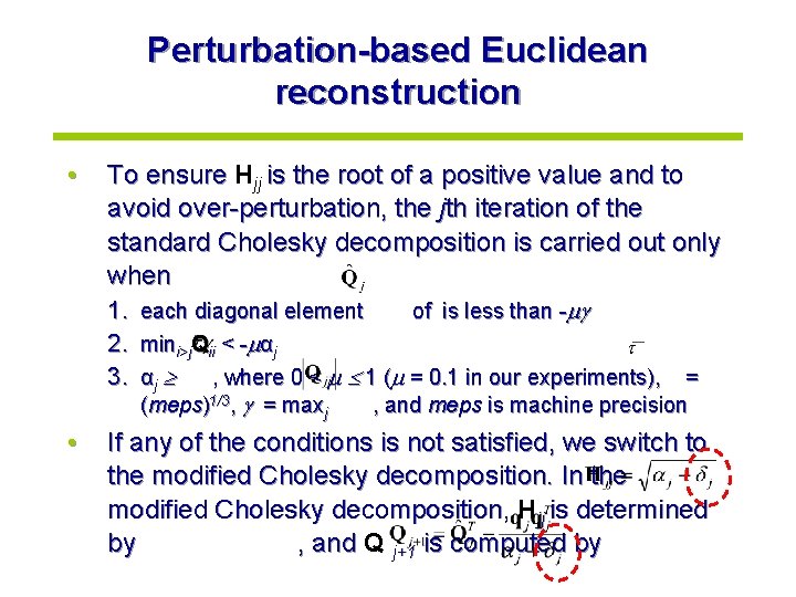
Perturbation-based Euclidean reconstruction • To ensure Hjj is the root of a positive value and to avoid over-perturbation, the jth iteration of the standard Cholesky decomposition is carried out only when 1. 2. 3. • each diagonal element of is less than - mini>j. Qii < - αj αj , where 0 < 1 ( = 0. 1 in our experiments), = (meps)1/3, = maxj , and meps is machine precision If any of the conditions is not satisfied, we switch to the modified Cholesky decomposition. In the modified Cholesky decomposition, Hjj is determined by , and Q j+1 is computed by

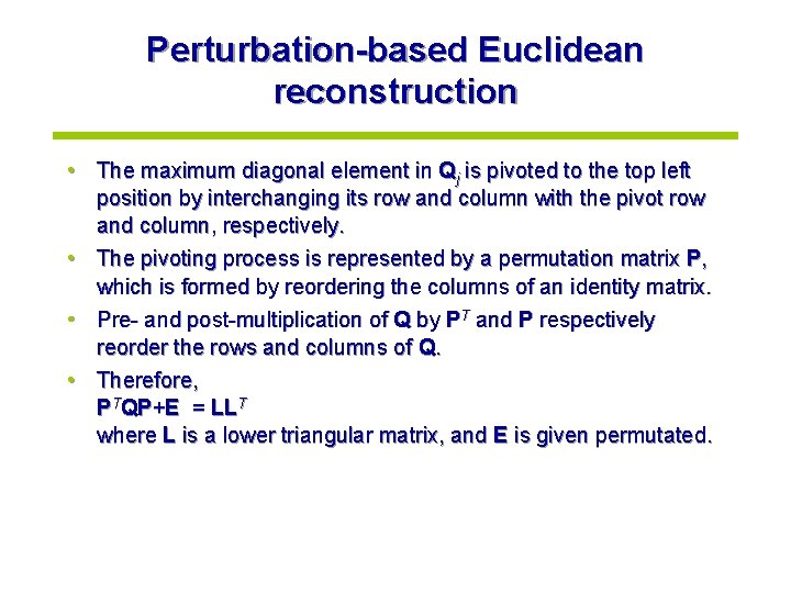
Perturbation-based Euclidean reconstruction • The maximum diagonal element in Qj is pivoted to the top left position by interchanging its row and column with the pivot row and column, respectively. • The pivoting process is represented by a permutation matrix P, which is formed by reordering the columns of an identity matrix. • Pre- and post-multiplication of Q by PT and P respectively reorder the rows and columns of Q. • Therefore, PTQP+E = LLT where L is a lower triangular matrix, and E is given permutated.

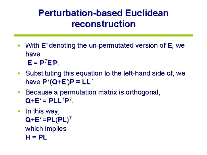
Perturbation-based Euclidean reconstruction • With E' denoting the un-permutated version of E, we have E = P TE ' P. • Substituting this equation to the left-hand side of, we have PT(Q+E')P = LLT. • Because a permutation matrix is orthogonal, Q+E' = PLLTPT. • In this way, Q+E' =PL(PL)T which implies H = PL

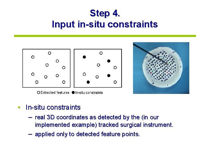
Step 4. Input in-situ constraints • In-situ constraints – real 3 D coordinates as detected by the (in our implemented example) tracked surgical instrument. – applied only to detected feature points.

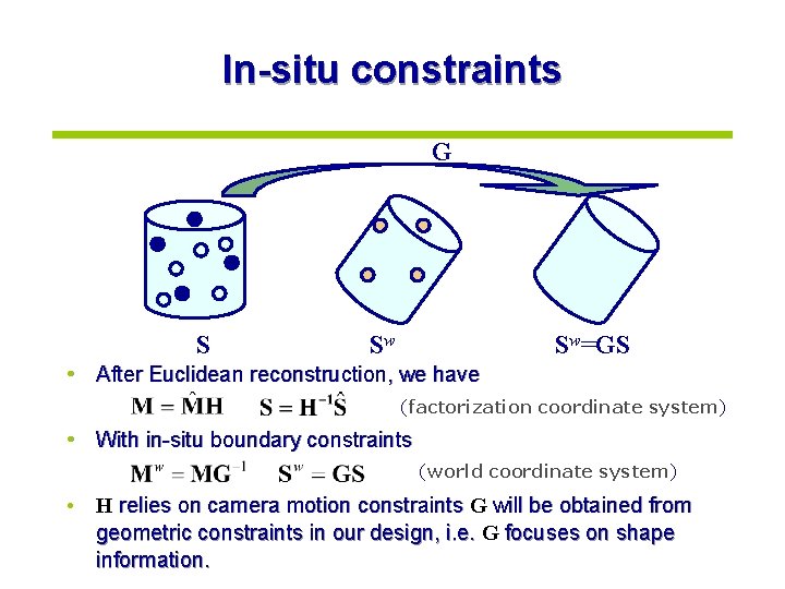
In-situ constraints G S Sw Sw=GS • After Euclidean reconstruction, we have (factorization coordinate system) • With in-situ boundary constraints (world coordinate system) • H relies on camera motion constraints G will be obtained from geometric constraints in our design, i. e. G focuses on shape information.

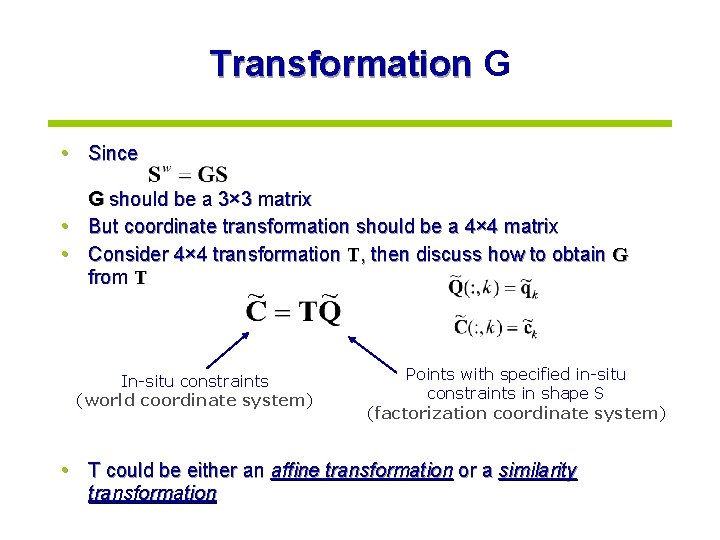
Transformation G • Since G should be a 3× 3 matrix • But coordinate transformation should be a 4× 4 matrix • Consider 4× 4 transformation T, then discuss how to obtain G from T In-situ constraints (world coordinate system) Points with specified in-situ constraints in shape S (factorization coordinate system) • T could be either an affine transformation or a similarity transformation

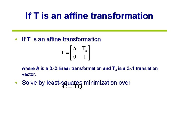
If T is an affine transformation • If T is an affine transformation where A is a 3 3 linear transformation and Ta is a 3 1 translation vector. • Solve by least-squares minimization over

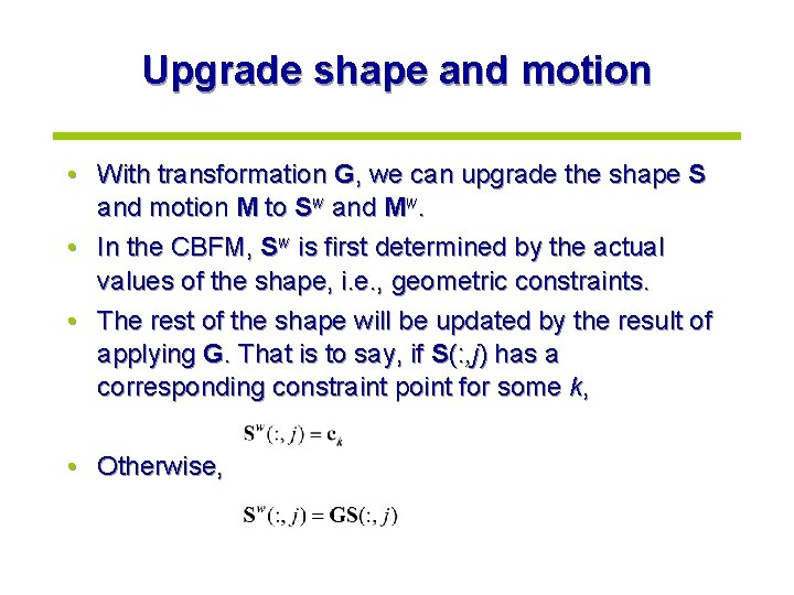
Upgrade shape and motion • With transformation G, we can upgrade the shape S and motion M to Sw and Mw. • In the CBFM, Sw is first determined by the actual values of the shape, i. e. , geometric constraints. • The rest of the shape will be updated by the result of applying G. That is to say, if S(: , j) has a corresponding constraint point for some k, • Otherwise,

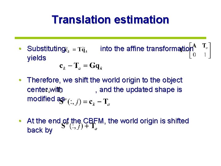
Translation estimation • Substituting yields into the affine transformation • Therefore, we shift the world origin to the object center with , and the updated shape is modified as • At the end of the CBFM, the world origin is shifted back by

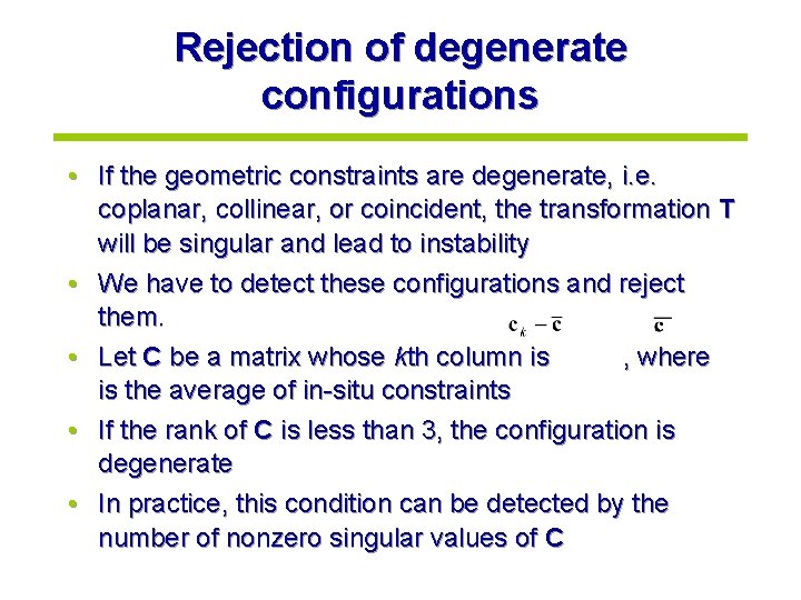
Rejection of degenerate configurations • If the geometric constraints are degenerate, i. e. coplanar, collinear, or coincident, the transformation T will be singular and lead to instability • We have to detect these configurations and reject them. • Let C be a matrix whose kth column is , where is the average of in-situ constraints • If the rank of C is less than 3, the configuration is degenerate • In practice, this condition can be detected by the number of nonzero singular values of C

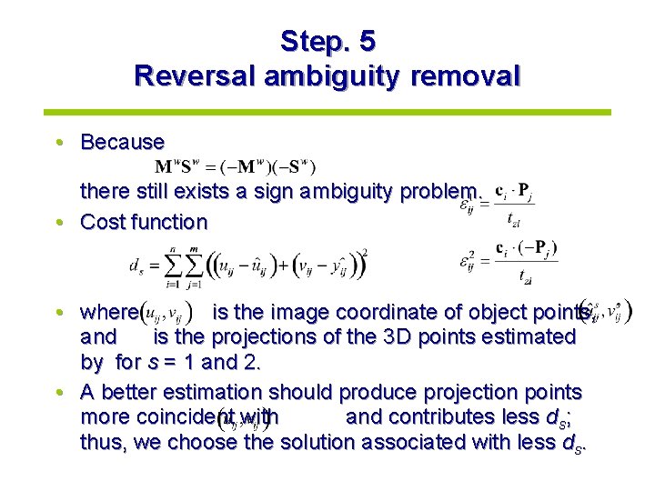
Step. 5 Reversal ambiguity removal • Because there still exists a sign ambiguity problem. • Cost function • where is the image coordinate of object points, and is the projections of the 3 D points estimated by for s = 1 and 2. • A better estimation should produce projection points more coincident with and contributes less ds; thus, we choose the solution associated with less ds.

In-situ routine

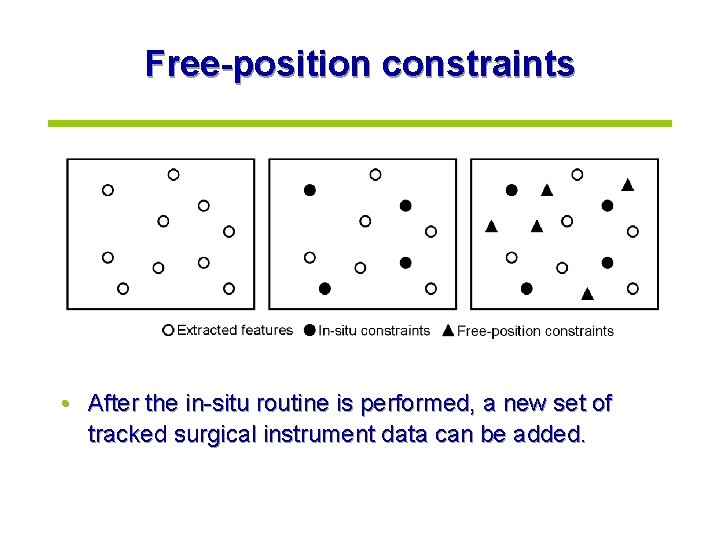
Free-position constraints • After the in-situ routine is performed, a new set of tracked surgical instrument data can be added.

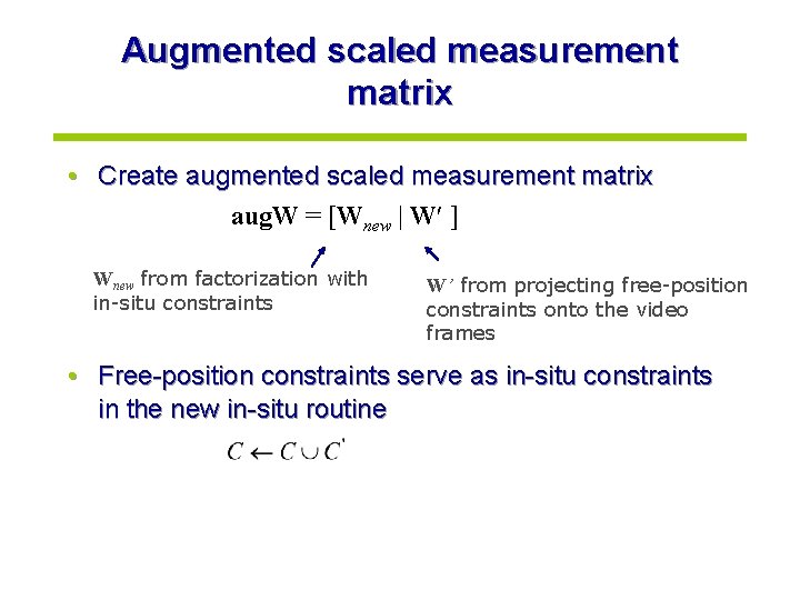
Augmented scaled measurement matrix • Create augmented scaled measurement matrix aug. W = [Wnew | W ] Wnew from factorization with in-situ constraints W’ from projecting free-position constraints onto the video frames • Free-position constraints serve as in-situ constraints in the new in-situ routine

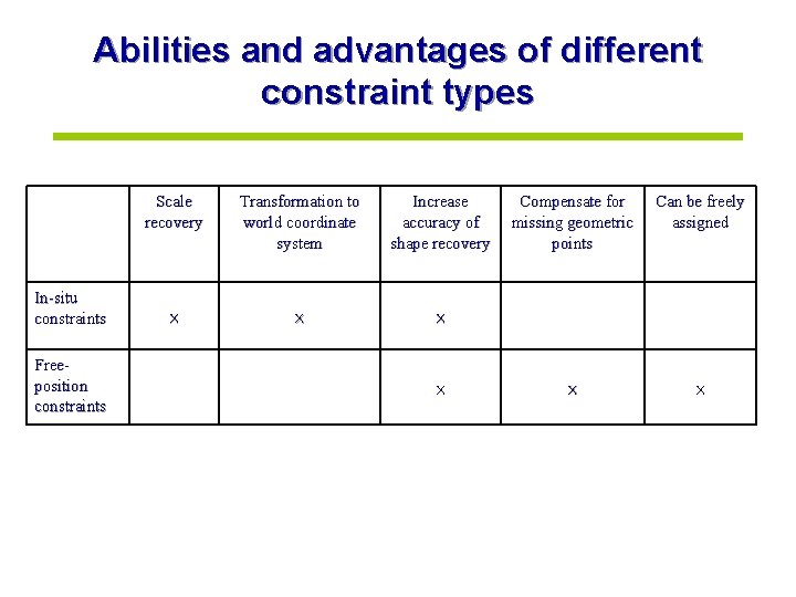
Abilities and advantages of different constraint types In-situ constraints Freeposition constraints Scale recovery Transformation to world coordinate system Increase accuracy of shape recovery × × Compensate for missing geometric points Can be freely assigned × ×

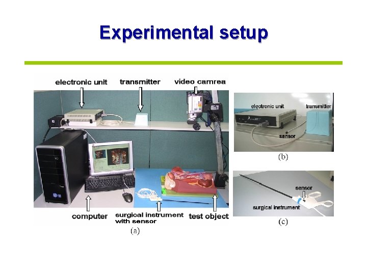
Experimental setup

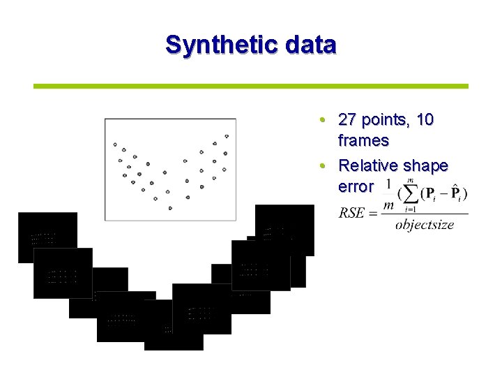
Synthetic data • 27 points, 10 frames • Relative shape error

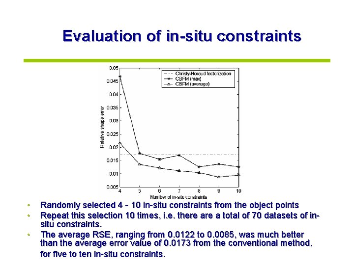
Evaluation of in-situ constraints • • • Randomly selected 4 - 10 in-situ constraints from the object points Repeat this selection 10 times, i. e. there a total of 70 datasets of insitu constraints. The average RSE, ranging from 0. 0122 to 0. 0085, was much better than the average error value of 0. 0173 from the conventional method, for five to ten in-situ constraints.

Evaluation of in-situ constraints • Because we replaced some estimated 3 D points by in-situ constraints and in-situ values can be assumed to be perfect, the shape error of these replaced points is zero. • If the rest of the shape is not improved, the RSE will still decrease. • To further demonstrate the ability to improve the overall shape, we re-calculate the RSE but exclude the points replaced by insitu constraints in order to achieve an objective evaluation. • The re-calculated average RSE ranges from 0. 0162 to 0. 0121, which is still better than the error value 0. 0185 from the conventional method, for five to ten constraints.

Evaluation of in-situ constraints scale recovery • If CBFM shape recovery is perfect then the recovered scale s 1 will equal 1 • We use |1 -s 1| as a measurement of scale error to evaluate scale recovery. • The average scale error |1 -s 1| is 0. 0016.

Evaluation of free-position constraints • • Randomly selected 10 point sets as test objects from the synthetic data, where each set has 20 points and their remaining 7 points are candidates for free-position constraints. For each test object, the computer randomly selected 1 7 free-position constraints from the candidates and four in-situ constraints from the object, where the RSE of these four in-situ constraints is used as the basis of comparison to demonstrate the performance of adding free-position constraints.

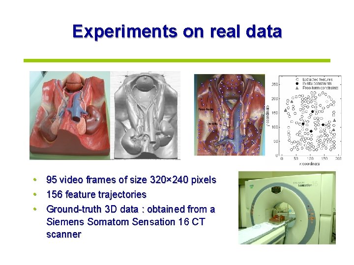
Experiments on real data • • • 95 video frames of size 320× 240 pixels 156 feature trajectories Ground-truth 3 D data : obtained from a Siemens Somatom Sensation 16 CT scanner

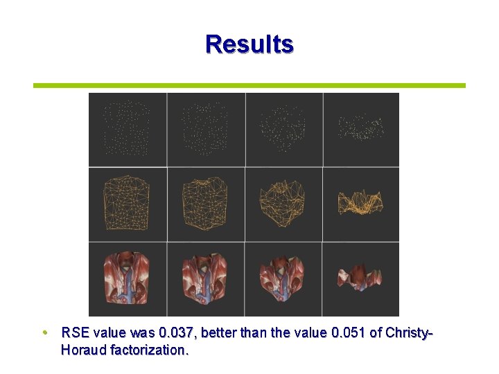
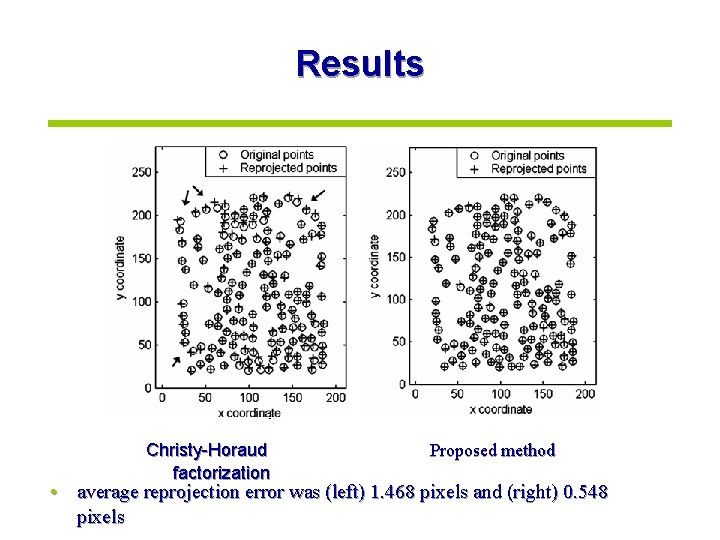
Results • RSE value was 0. 037, better than the value 0. 051 of Christy. Horaud factorization.

Results Christy-Horaud factorization Proposed method • average reprojection error was (left) 1. 468 pixels and (right) 0. 548 pixels

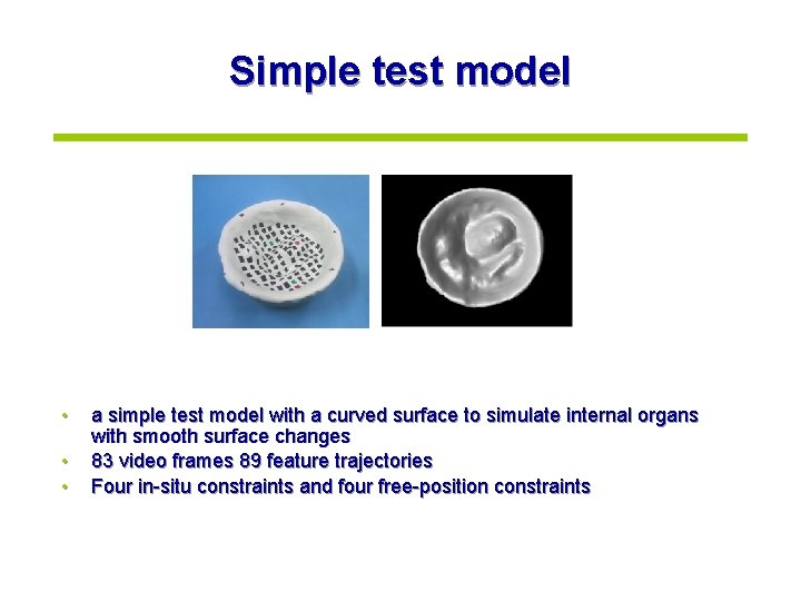
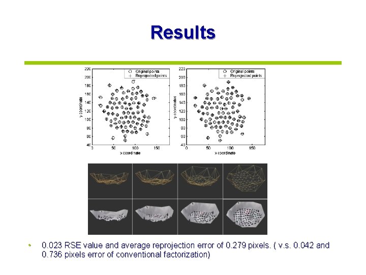
Simple test model • • • a simple test model with a curved surface to simulate internal organs with smooth surface changes 83 video frames 89 feature trajectories Four in-situ constraints and four free-position constraints

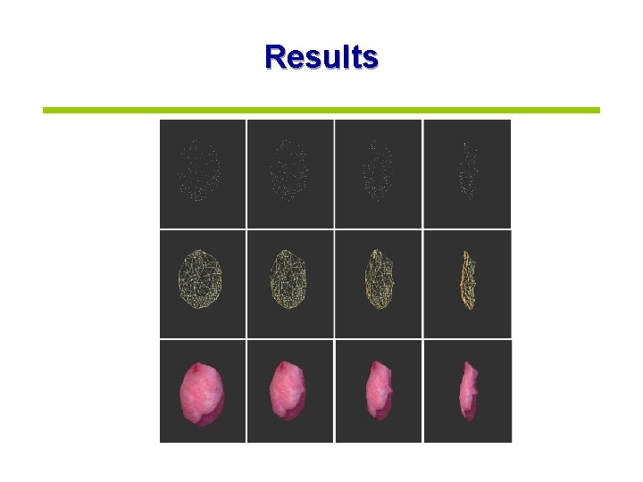
Results • 0. 023 RSE value and average reprojection error of 0. 279 pixels. ( v. s. 0. 042 and 0. 736 pixels error of conventional factorization)

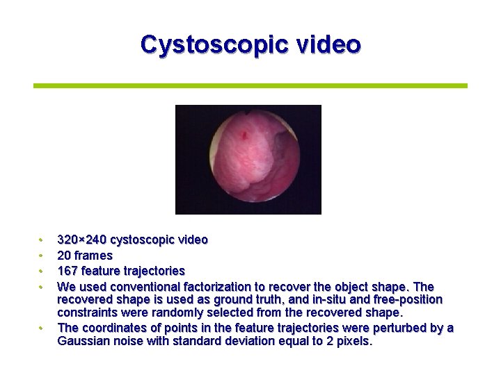
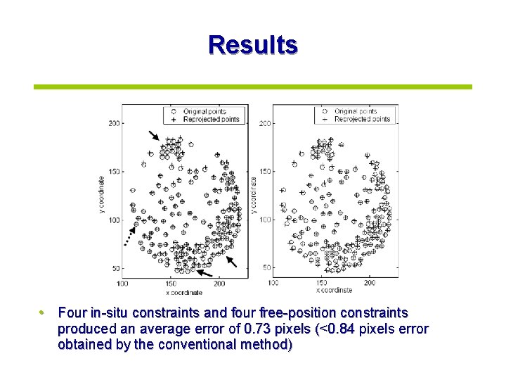
Cystoscopic video • • • 320× 240 cystoscopic video 20 frames 167 feature trajectories We used conventional factorization to recover the object shape. The recovered shape is used as ground truth, and in-situ and free-position constraints were randomly selected from the recovered shape. The coordinates of points in the feature trajectories were perturbed by a Gaussian noise with standard deviation equal to 2 pixels.

Results • Four in-situ constraints and four free-position constraints produced an average error of 0. 73 pixels (<0. 84 pixels error obtained by the conventional method)

Results

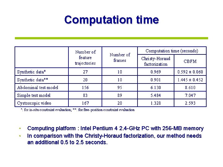
Computation time Number of feature trajectories Number of frames Synthetic data* 27 Synthetic data** Computation time (seconds) Christy-Horaud factorization CBFM 10 0. 969 0. 592 ± 0. 060 20 10 0. 901 1. 445 ± 0. 452 Abdominal test model 156 95 6. 130 8. 610 Simple test model 83 89 5. 484 7. 047 Cystoscopic video 167 20 1. 328 2. 593 *: for in-situ constraint evaluation; **: for free-position constraint evaluation • • Computing platform : Intel Pentium 4 2. 4 -GHz PC with 256 -MB memory In comparison with the Christy-Horaud factorization, our method needs an additional 0. 5 to 2. 5 seconds.

Conclusions • The CBFM combines normal 2 D endoscopic video and 3 D positioning technology for recovering human inner structures without any high-cost medical imaging • It utilizes matrix decomposition to separate the feature trajectories, generated from a software pipeline for feature tracking, in order to estimate the motion of the camera and the shape of the target • Two kinds of geometric constraints were presented: in-situ and free-position, where in-situ constraints are obtained by feature positioning, and free-position constraints deal with the non-feature portion

Conclusions • We also propose a new perturbation-based Euclidean reconstruction that successfully solves the non-positive definite problem in a non-parametric way • Experiments on both real and simulated data demonstrate that this method is more accurate than the conventional method and the object scale is preserved

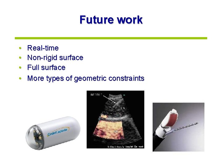
Future work • • Real-time Non-rigid surface Full surface More types of geometric constraints

Thank you!