Computer Vision Feature Detection Computer Vision Outline 1

Computer Vision Feature Detection

Computer Vision Outline 1. Edge detection a. Gradient operators b. Zero-crossings of Laplacians c. Canny Edge Detector 2. Corner detection

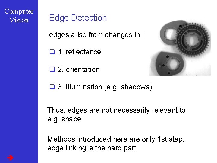
Computer Vision Edge Detection edges arise from changes in : q 1. reflectance q 2. orientation q 3. Illumination (e. g. shadows) Thus, edges are not necessarily relevant to e. g. shape Methods introduced here are only 1 st step, edge linking is the hard part

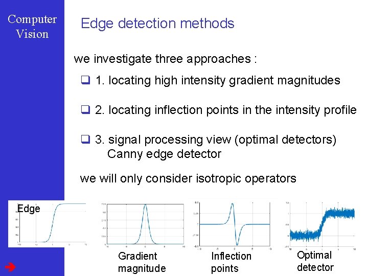
Computer Vision Edge detection methods we investigate three approaches : q 1. locating high intensity gradient magnitudes q 2. locating inflection points in the intensity profile q 3. signal processing view (optimal detectors) Canny edge detector we will only consider isotropic operators Edge Gradient magnitude Inflection points Optimal detector

Computer Vision Gradient operators : principle image ƒ(x, y) : locate edges at ƒ’s steep slopes measure the gradient magnitude easy to check that this operator is isotropic the direction of steepest change : rotate coordinate frame and find that maximizes differentiation w. r. t. yields the corresponding magnitude is the one defined above

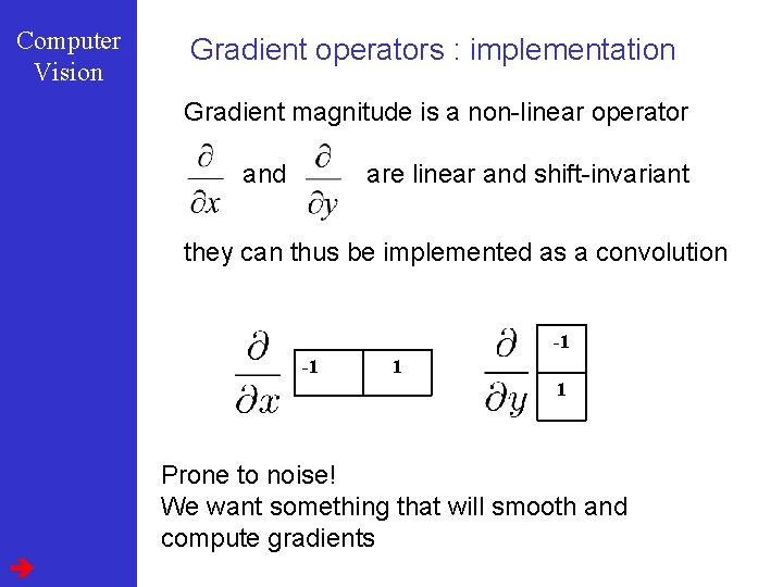
Computer Vision Gradient operators : implementation Gradient magnitude is a non-linear operator and are linear and shift-invariant they can thus be implemented as a convolution -1 -1 1 1 Prone to noise! We want something that will smooth and compute gradients

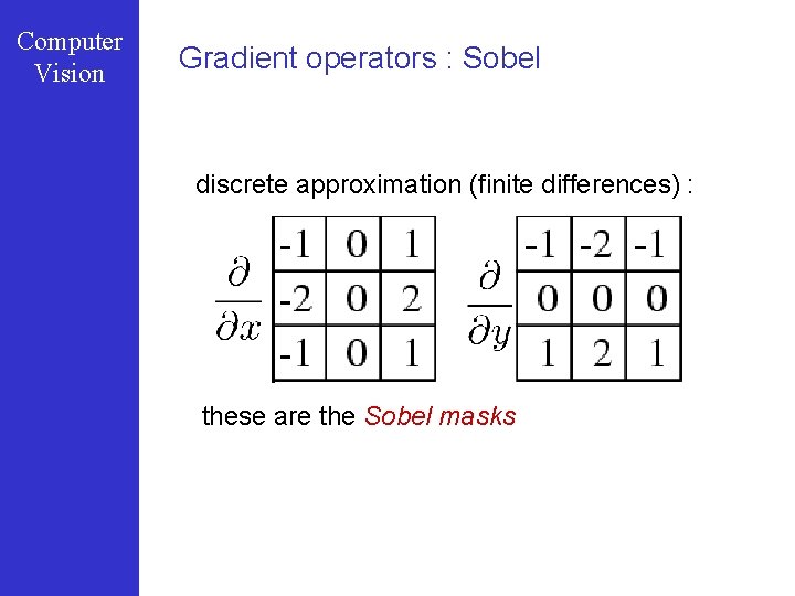
Computer Vision Gradient operators : Sobel discrete approximation (finite differences) : these are the Sobel masks

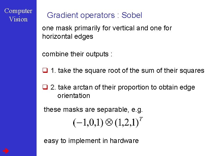
Computer Vision Gradient operators : Sobel one mask primarily for vertical and one for horizontal edges combine their outputs : q 1. take the square root of the sum of their squares q 2. take arctan of their proportion to obtain edge orientation these masks are separable, e. g. easy to implement in hardware

Computer Vision Gradient operators : MTF shows smoothing effect of Sobel mask example : MTF of the vertical Sobel mask this is a pure imaginary function, resulting in /2 phase shifts power spectrum : u-dir. : band-pass, v-dir. : low-pass

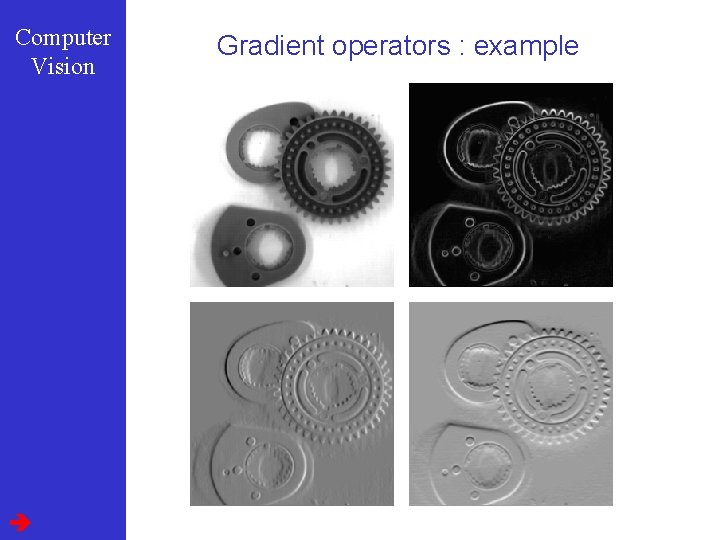
Computer Vision Gradient operators : example

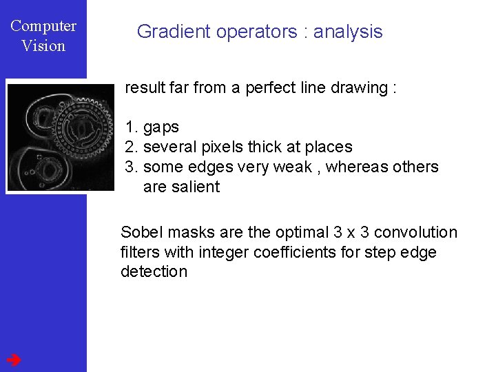
Computer Vision Gradient operators : analysis result far from a perfect line drawing : 1. gaps 2. several pixels thick at places 3. some edges very weak , whereas others are salient Sobel masks are the optimal 3 x 3 convolution filters with integer coefficients for step edge detection

Computer Vision Outline 1. Edge detection a. Gradient operators b. Zero-crossings of Laplacians c. Canny Edge Detector 2. Corner detection

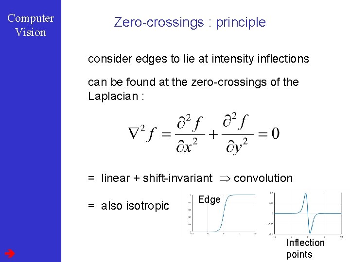
Computer Vision Zero-crossings : principle consider edges to lie at intensity inflections can be found at the zero-crossings of the Laplacian : = linear + shift-invariant convolution = also isotropic Edge Inflection points

Computer Vision Discrete approximations of the Laplacian MTF of left filter : MTF’s

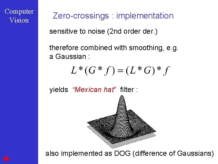
Computer Vision Zero-crossings : implementation sensitive to noise (2 nd order der. ) therefore combined with smoothing, e. g. a Gaussian : yields “Mexican hat” filter : also implemented as DOG (difference of Gaussians)

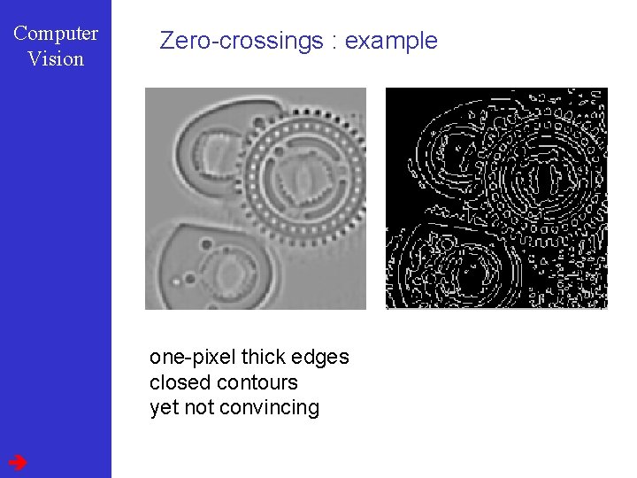
Computer Vision Zero-crossings : example one-pixel thick edges closed contours yet not convincing

Computer Vision Outline 1. Edge detection a. Gradient operators b. Zero-crossings of Laplacians c. Canny Edge Detector 2. Corner detection

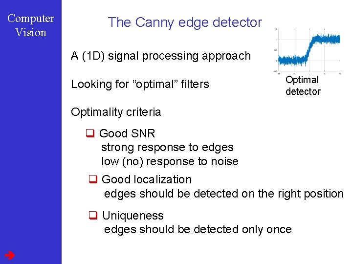
Computer Vision The Canny edge detector A (1 D) signal processing approach Looking for “optimal” filters Optimal detector Optimality criteria q Good SNR strong response to edges low (no) response to noise q Good localization edges should be detected on the right position q Uniqueness edges should be detected only once

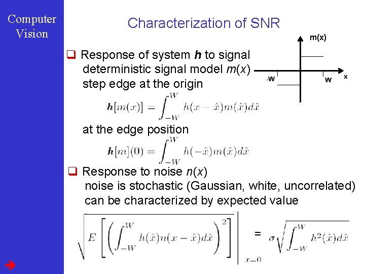
Computer Vision Characterization of SNR m(x) q Response of system h to signal deterministic signal model m(x) step edge at the origin -W W x at the edge position q Response to noise n(x) noise is stochastic (Gaussian, white, uncorrelated) can be characterized by expected value =

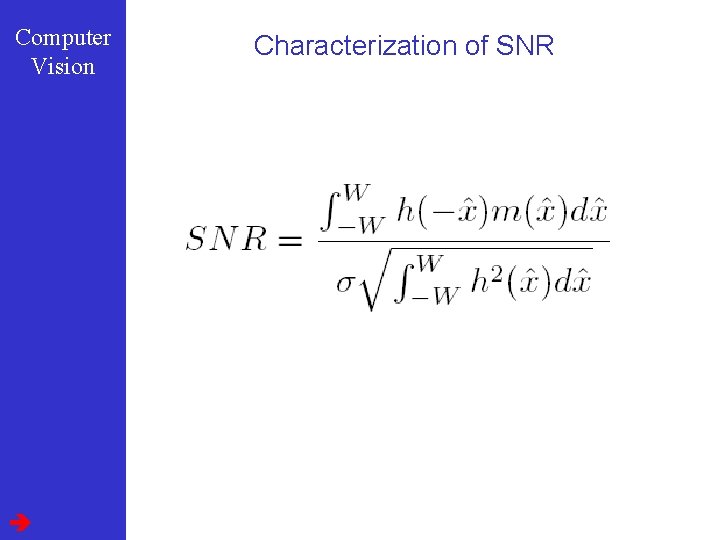
Computer Vision Characterization of SNR

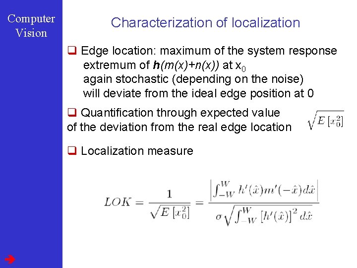
Computer Vision Characterization of localization q Edge location: maximum of the system response extremum of h(m(x)+n(x)) at x 0 again stochastic (depending on the noise) will deviate from the ideal edge position at 0 q Quantification through expected value of the deviation from the real edge location q Localization measure

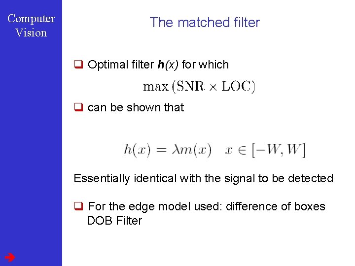
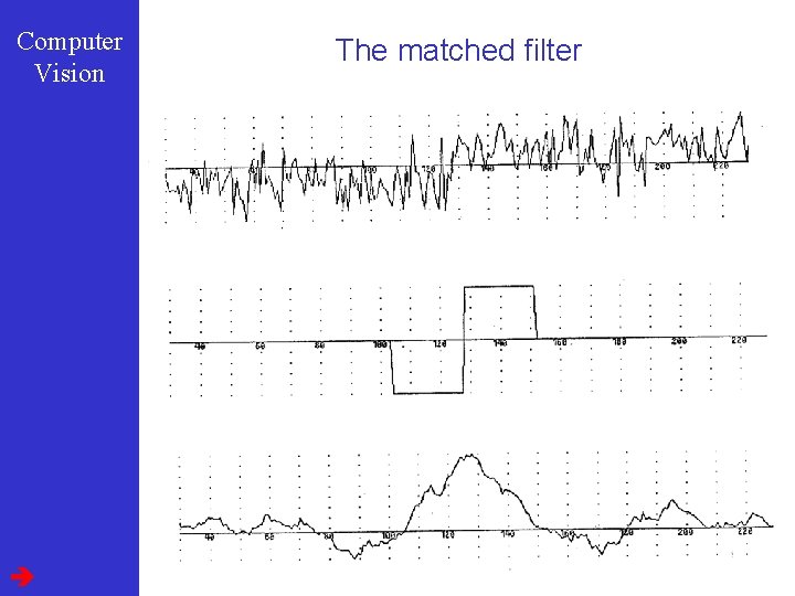
Computer Vision The matched filter q Optimal filter h(x) for which q can be shown that Essentially identical with the signal to be detected q For the edge model used: difference of boxes DOB Filter

Computer Vision The matched filter

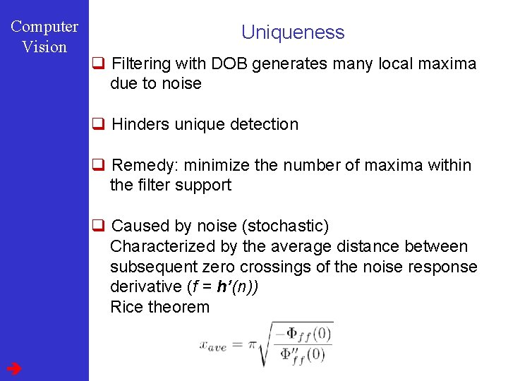
Computer Vision Uniqueness q Filtering with DOB generates many local maxima due to noise q Hinders unique detection q Remedy: minimize the number of maxima within the filter support q Caused by noise (stochastic) Characterized by the average distance between subsequent zero crossings of the noise response derivative (f = h’(n)) Rice theorem

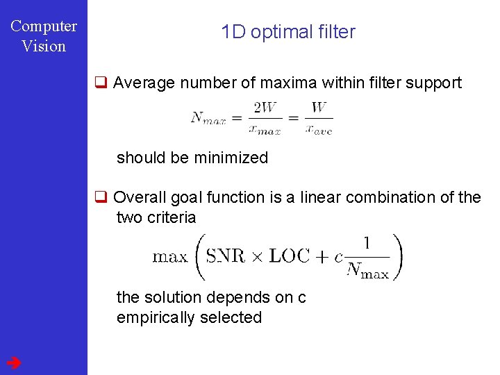
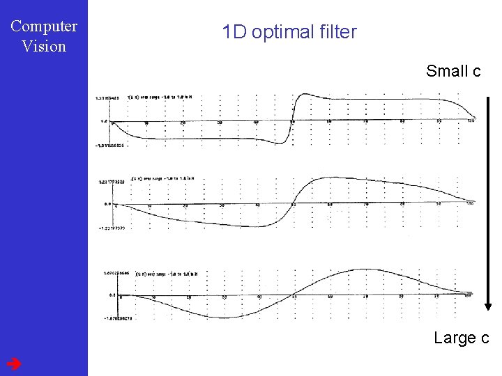
Computer Vision 1 D optimal filter q Average number of maxima within filter support should be minimized q Overall goal function is a linear combination of the two criteria the solution depends on c empirically selected

Computer Vision 1 D optimal filter Small c Large c

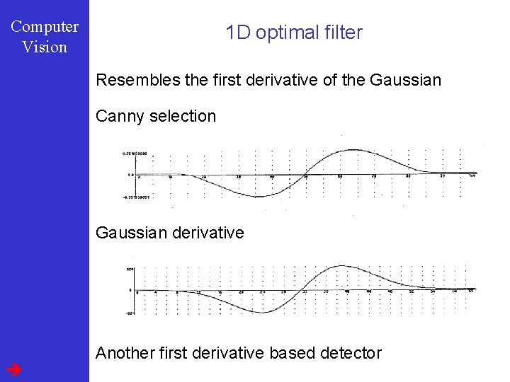
Computer Vision 1 D optimal filter Resembles the first derivative of the Gaussian Canny selection Gaussian derivative Another first derivative based detector

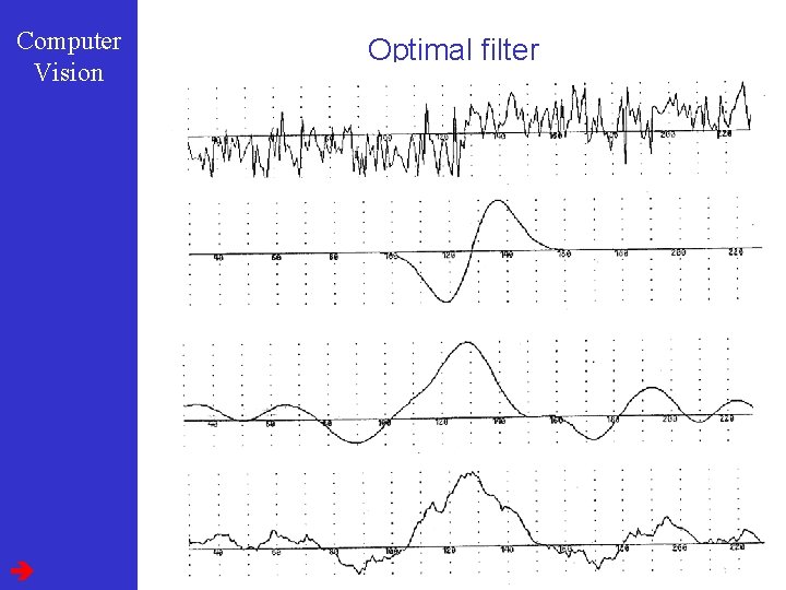
Computer Vision Optimal filter

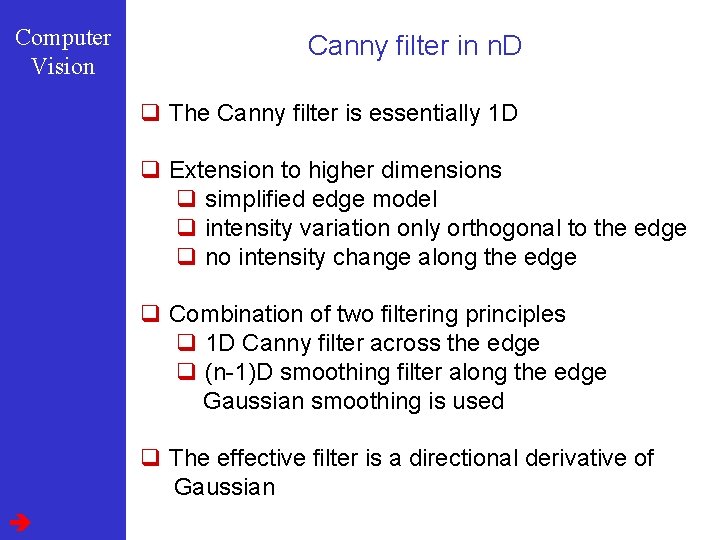
Computer Vision Canny filter in n. D q The Canny filter is essentially 1 D q Extension to higher dimensions q simplified edge model q intensity variation only orthogonal to the edge q no intensity change along the edge q Combination of two filtering principles q 1 D Canny filter across the edge q (n-1)D smoothing filter along the edge Gaussian smoothing is used q The effective filter is a directional derivative of Gaussian

Computer Vision The 2 D Canny filter

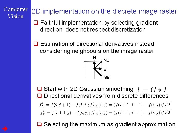
Computer 2 D implementation on the discrete image raster Vision q Faithful implementation by selecting gradient direction: does not respect discretization q Estimation of directional derivatives instead considering neighbours on the image raster N NE E SE q Start with 2 D Gaussian smoothing q Directional derivatives from discrete differences q Selecting the maximum as gradient approximation

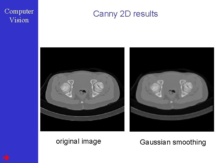
Computer Vision Canny 2 D results original image Gaussian smoothing

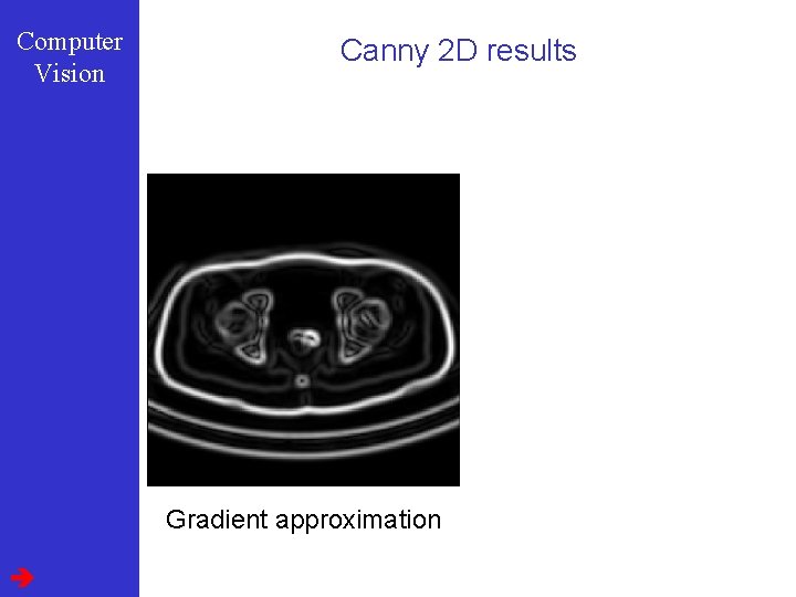
Computer Vision Canny 2 D results Gradient approximation

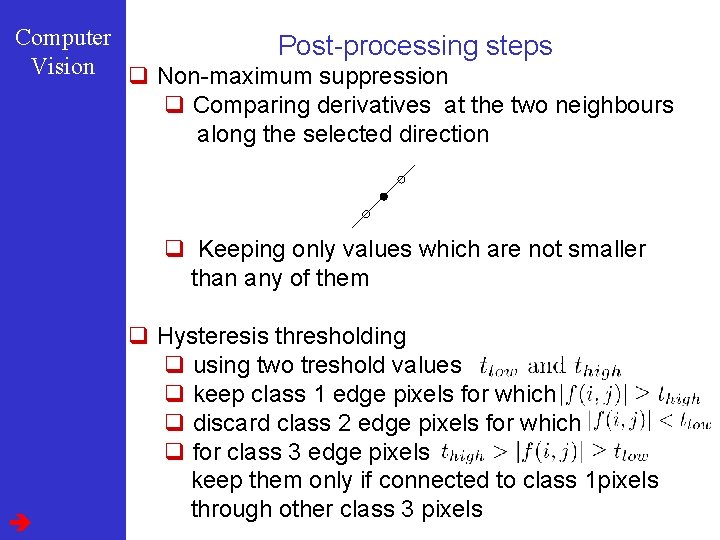
Computer Post-processing steps Vision q Non-maximum suppression q Comparing derivatives at the two neighbours along the selected direction q Keeping only values which are not smaller than any of them q Hysteresis thresholding q using two treshold values q keep class 1 edge pixels for which q discard class 2 edge pixels for which q for class 3 edge pixels keep them only if connected to class 1 pixels through other class 3 pixels

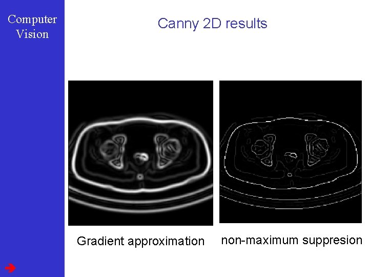
Computer Vision Canny 2 D results Gradient approximation non-maximum suppresion

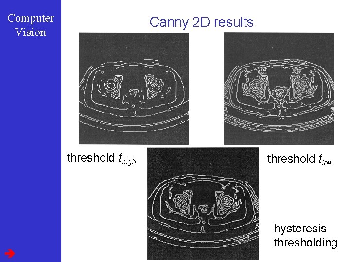
Computer Vision Canny 2 D results threshold thigh threshold tlow hysteresis thresholding

Computer Vision Remarks to the Canny filter q The state-of-the-art edge detector even today q Very efficient implementation no interpolation is needed as respecting the raster q Post-processing is the major contribution q Can be applied to any gradient-based edge detection scheme q Fails where the simplified edge model is wrong q crossing, corners, … q gaps can be created q mainly due to non-maximum suppression q Hysteresis thresholding is only effective in 2 D

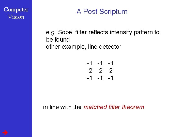
Computer Vision A Post Scriptum e. g. Sobel filter reflects intensity pattern to be found other example, line detector -1 -1 -1 2 2 2 -1 -1 -1 in line with the matched filter theorem

Computer Vision Outline 1. Edge detection a. Gradient operators b. Zero-crossings of Laplacians c. Canny Edge Detector 2. Corner detection

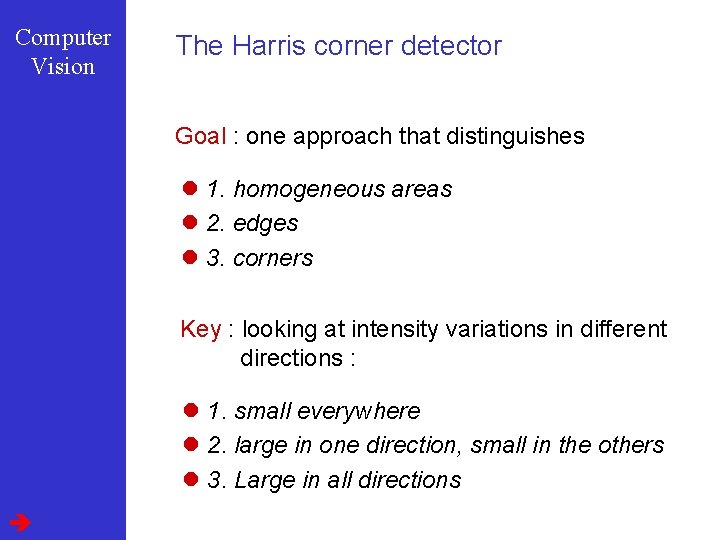
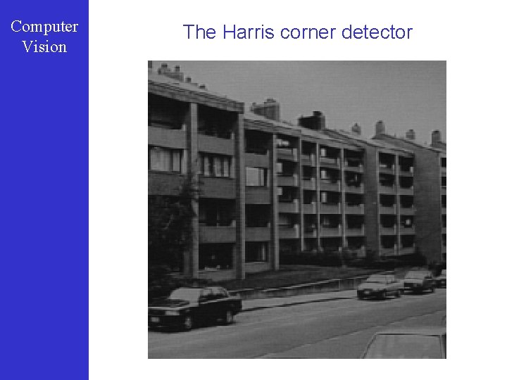
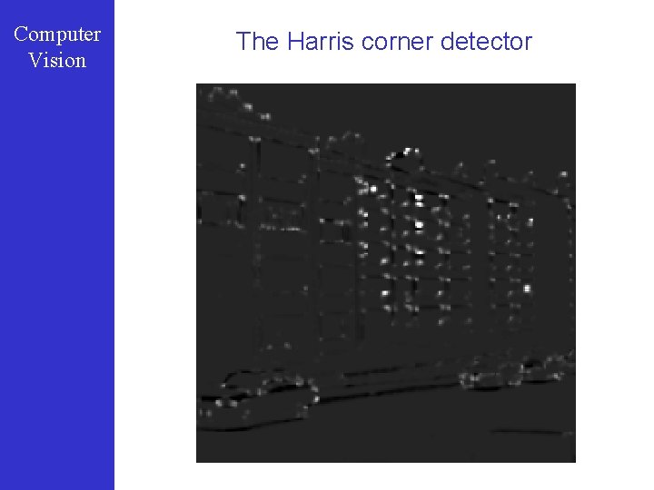
Computer Vision The Harris corner detector Goal : one approach that distinguishes l 1. homogeneous areas l 2. edges l 3. corners Key : looking at intensity variations in different directions : l 1. small everywhere l 2. large in one direction, small in the others l 3. Large in all directions

Computer Vision The Harris corner detector Homogeneous region Edge region Corner region Approach : find the directions of minimal and maximal change Second order moments of the intensity variations : Look for the eigenvectors and eigenvalues

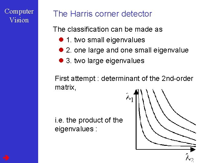
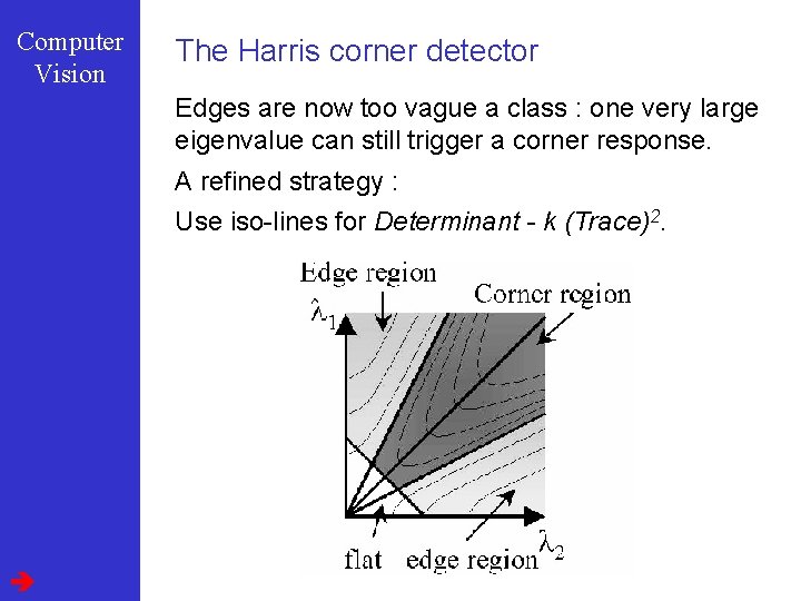
Computer Vision The Harris corner detector The classification can be made as l 1. two small eigenvalues l 2. one large and one small eigenvalue l 3. two large eigenvalues First attempt : determinant of the 2 nd-order matrix, i. e. the product of the eigenvalues :

Computer Vision The Harris corner detector Edges are now too vague a class : one very large eigenvalue can still trigger a corner response. A refined strategy : Use iso-lines for Determinant - k (Trace)2.

Computer Vision The Harris corner detector

Computer Vision The Harris corner detector