DC Spark Experiments 10092020 What are the CERN

DC Spark Experiments 10/09/2020

What are the CERN DC spark systems? The CERN DC spark systems consist of an anode and cathode in a rod-plane geometry in ultrahigh vacuum. I will be talking about system I which is powered by the High-Rep-Rate circuit. The gap size can be varied from 0 -100 um by using a stepper motor. It is possible to monitor and actively control the gap with an accuracy of ~1. 5 um. The diameter of the anode is 2. 3 mm and has a hemispherical tip. High voltage is applied across the electrodes and the resulting current and voltage waveforms are analysed (largely automatically) and recorded. The cathodes have a good surface quality. From these we can tell whether a BD occurred and measure several properties of the BD such as the turn on time, the position of the BD within the pulse, the burning voltage and even the gap distance! We are not currently able to measure the field enhancement factor β, with this setup however. 2

What is the Fixed Gap System Despite the comparatively large size of the anodes, the system is very compact. Four antennas are included in the design to pick up the radiation from breakdowns. The surface of the electrodes are 60 mm in diameter and have a shape tolerance of <1 um. The picture on the right shows the high precision turning. 3

Motivation behind the fixed gap system This fixed gap system solves two key issues… 1. There is no need to measure the electrode gap, it is fixed. 2. The surface area is very much larger, so hopefully breakdown will usually occur on “virgin” surface which hasn’t seen a breakdown yet. Also the system is very compact 30 cm x 30 cm. This will allow the whole system to be placed inside a 2 T magnet we have at CERN, enabling us to study the effect an external magnetic field has on the BDR. These SEM pictures well illustrate the difference in experimental conditions in RF tests (Right) which even after 100 s of hours of testing shows minimal surface modification compared to just 5 breakdowns in the present DC spark system (Left). 4

What is the High Rep Rate Circuit? The HRR circuit uses a solid state switch to supply high voltage pulses (up to 10 k. V) at a rep rate of up to 1 k. Hz. The energy is stored on a 200 m/1 us long coaxial cable. The picture above shows the HRR circuit. The metal box housing the switch is placed as close as possible to the vacuum chamber to minimise stray capacitance. 5

The High Rep Rate System 6

Measured traces • Fast voltage rise, but slow voltage fall time • Pulse length adjustments not useful • Small and brief initial charging current • The turn on time is how quickly the voltage drops after a BD. • The BD position is the position or time the BD occurs within the pulse. • An estimation of the burning voltage can be obtained by averaging the voltage fluctuations after the BD.

BD statistics at fixed voltage

BDR Analysis of long run in Sys I Total #BDs 972 Average BDR 2. 95*10^-5 BDs/pulse Std(pulses between BD) 8. 54*10^4 Ratio(immediate BDs/Total BDs) 0. 64 • Clusters mean the calculated BDR for 20 BDs may not reflect the underlying BDR. • BDR fluctuates but no conditioning is seen.

BDR Analysis of long run in Sys I This experiment was performed at a surface electric field of 170 MV/m and a gap size of 20 um. The large number of BDs which occur immediately following a previous BD cause the data to deviate significantly from the Poisson distribution that might otherwise be expected. Total #BDs 972 Average BDR 2. 95*10^-5 BDs/pulse Std(pulses between BD) 8. 54*10^4 Ratio(immediate BDs/Total BDs) 0. 64

Conditioning in FGS Cluster ratio = 0. 47 Cluster ratio = 0. 25 The flattening of these curves is evidence of conditioning. The BDR increases sharply when the voltage is increased. The cluster ratio define as BDs in a cluster/Total BDs is higher for higher BDRs.

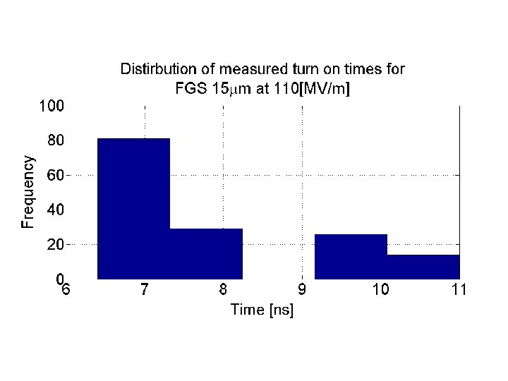
FGS Poisson 110 MV/m #BDs BDR Ratio immediate BDs/Total BDs 177 1. 5*10^-6 0. 40 The distribution of BDs is not Poissonian even when clusters have been removed.

BDR vs E

BDR vs E 14 um and 25 um gap For each experiment the gap is first set to the required distance. Then the voltage is set at the highest value and the HRR circuit begins pulsing at 1000 Hz. After 100 BDs have been recorded or 10^7 pulses and at least 10 BDs the voltage is reduced by 5%. Every 10 mins if no BD has occurred the HRR circuit is made to pulse at a predetermined voltage too low for a BD to occur, so the gap can be measured and automatically corrected. As the uncertainty in the gap is always around 2 um the error in the field is much larger at smaller gap sizes.

BDR vs E 40 um gap Both the power law model and the stress model fit the data well. Going to a lower BDR in the future should help distinguish between them. The exponents obtained for the power law model are very similar to those obtained in high power RF tests of accelerating cavities. The fitted exponent tends to decrease for a larger gap.

The Fixed Gap System BDR ~ E^45 BDR ~ E^40 First voltage was decreased in steps of 5% (red). Once a BDR of ~5*10^-8 was achieved the voltage was increased in steps of 5% (blue). The electrodes have conditioned so the BDR data in blue is consistently lower than the BDR data in red.

Time until BD

Distribution of Time until BD Histogram of time until BD Almost all BDs occur at the beginning of the pulse. The distribution of non immediate BDs is quite flat up to 3 us at which point the voltage across the gap begins to fall. A small drop in voltage due to a reflection from the end of the PFL results in fewer BDs at 2 us.

Time until BD dependencies The position of the BD within the pulse, in some experiments, is seen to occur later for lower fields and BDRs. The graph below shows some old data taken at a gap of 20 um but before gap monitoring was possible.

FGS Time until BD The distribution of the time until BD is peaked at shorter times. However it is not as strongly peaked as it was in system I. Due to the higher capacitance between the electrodes BDs are also able to occur later than in sys. I and the effect of the fluctuations in the voltage pulse can be seen more strongly. In the bottom plot the voltage pulse can be seen in blue a BD occurs at the time denoted as 0 us. In this case the time until BD was around 3 us.

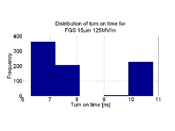
FGS Time until BD BDs that happen within a cluster are far more likely to have a shorter time until BD than BDs which do not happen within a cluster. Again the field in this case was 125 MV/m.

FGS Time until BD 8 By taking a rolling average of 50 points it can be seen that the average time until BD shows a slight tendency to increase. As the electrodes condition. The electric field in this case was always 125 MV/m.

Measured Turn on Times 23

Turn on time measured in the DC Spark system The turn on time appears uncorrelated with gap size or BD position, but is generally higher at higher surface fields.

Comparison of falling edge duration The Swiss FEL turn on times are much longer than in the DC case and the variation is much greater, this is keeping with other RF breakdown turn on time measurements. Test Measurement Simulation The summary table on the right suggests the characteristic size of the system breaking down may govern the turn on time. Result ~0. 5 ns… maybe see Kyrre’s talk New DC System Voltage Fall Time ~7 ns TBTS (X-Band) Transmitted Power Fall Time 20 -40 ns KEK (X-Band) Transmitted Power Fall Time 20 -40 ns Swiss FEL (C-Band) Transmitted Power Fall Time 110 -140 ns 25

Measured Burning Voltages 26

Measured Burning Voltages The burning voltage was measured across here. It is the “steady state” voltage across the plasma of a spark during a breakdown at which point most of the voltage is dropped across the 50 Ohm resistor. It is a property of the material. Subtract average voltage with switch closed from Average voltage during breakdown after initial voltage fall. 27

Measured Burning Voltages The literature gives a value for the burning voltage of clean copper of ~23 V. This is lower than what I have measure so far in the DC spark system. But I have not measured or corrected for the short circuit resistance of cables etc. The low burning voltage indicates the arc has a very low impedance, with this external circuit and voltage the impedance was ~0. 5 Ohm. 28

BDR Dependence on Pulse Width 29

Changing the pulse width • The voltage pulse can be adjusted by changing the length of time for which the switch remains closed. • The bleed resistors circled in red were replaced with smaller ones so that the voltage would decay faster after the switch is opened. It takes around 200 ns for the voltage to decay to 90%. • Taking into account the time to decay to 90% the pulse width can be adjusted between ~300 ns and ~7 us.

Pulse Width vs. BDR If these results prove to be repeatable they are quite remarkably close to the behavior observed in RF accelerating cavities. Despite the much longer pulse lengths and very different geometry. Before these experiments I was of the opinion that the BDR~t^6 scaling law observed in RF was somehow related to the number of RF cycles and we would therefore not see an effect in a DC experiment. This was a reasonable guess especially considering the vast majority of DC breakdowns happen right at the beginning of the pulse as opposed to in accelerating structures where they are more evenly spread.

Effect of static magnetic field on the BDR in the FGS • The FGS was placed in a large electromagnet which could generate a magnetic field up to 0. 5 T. • The system was left running at a fixed voltage and the magnet was alternately switch on and then off again. • The analysis of the data is still ongoing but it looks as if any effect is small and within statistical errors. • The lack of an effect may be explained by the small distance between the electrodes of the FGS.

Effect of Magnetic Field Perpendicular To Electrodes – 15 um Blue is without field red is with 0. 5 T parallel to electrodes. Is the BDR consistently higher with field?

Summary • The HRR circuit enables us to study the dependency of BDR on Field and Pulse Length as well as the distribution of BDs, time until BD and turn on time at very low BDRs. • No significant differences have been found between RF breakdowns and DC breakdowns which makes the study of DC breakdown extremely useful for CLIC. • The FGS even behaves like an RF structure in terms of conditioning and once scaled for Pulse Length even the surface field for a given BDR is remarkably similar. • In addition the HRR circuit now allows us to operate at 1 k. Hz allowing us to generate data at 200 times the rate possible in a high power RF test. • In the future more precise measurements and detailed analysis will provide useful information for high power RF testing and perhaps even structure design. • Details on future plans for the DC Breakdown experiments will be given by Tomoko and Anders in a moment.

Back Up Slides

Monitoring of electrode gap

Pulse Integration Method The pulse integration method is used to monitor the gap distance. Current transformer 2 as shown in the circuit diagram is used to measure the transient current flow when the switch is closed. The area of this current pulse is dependent on the gap capacitance. In this position the current transformer is insensitive to as much stray capacitance as possible CT 2 5 ns/div The measurement used is an average of many pulses. 1μs/div

Calibration Curve A cubic function is fitted to the calibration data and used to convert subsequent integral measurements to a gap distance. How good is the measurement? We are able to measure the gap to +-1. 5 um, as yet it hasn’t been determined if this is a limit on the gap measurement or the gap tends to actually vary by this amount. The error introduced when going into contact is of the order of 1 um, but this only introduces a fixed offset.

Change in Gap without BDs The system was left pulsing at 100 Hz 2000 V for a day in order to measure the gap variation with no BDs over time. This plot was generated from the data in the previous plot it shows ΔX against ΔT, where: ΔX(ΔT) = mean(abs(d(t) – d(t+ ΔT)), over all t And d(t) is the measured gap distance at time t

Change in Gap with BDs V Std 7 k. V 0. 82 um 8. 5 k. V 0. 92 um 10 k. V 1. 22 um 11. 5 k. V 2. 75 um Interestingly although it is not obvious by eye the change in gap after BD does appear to be correlated to the BD voltage. In this plot each point represents a gap measurement @2000 V after a single BD was forced to occur at a higher voltage indicated in the legend. The gap was not reset by going into contact after each series. Oddly the gap appears to suddenly get smaller at 11. 5 k. V.

Turn on Time FGS

Explanation of magnet results

Explanation of magnet results • What made us study BD with an external magnetic field? And can we explain the lack of observed dependence? • For ionisation cooling a muon collider would require normal conducting RF cavities that can operate at “high” gradient within a magnetic field strength of up to approximately 6 T. • Mu. Cool is an experiment studying the effect of the magnetic field on an 801 MHz pillbox cavity. • They see a substantial decrease in operating gradient with a field strength of ~3 T and a small but noticeable difference even with 0. 5 T. • They DON’T see any effect when they fill their cavities with high pressure hydrogen. 45

Figure on left shows the maximum achievable gradient for evacuated 801 MHz copper pillbox cavity wrt magnetic field. There is small but noticeable effect even at 0. 5 T. Figure below shows there is no difference between the achievable gradient of a similar Mo cavity when it is filled with high pressure (20 -100 atm) H gas. This was explained as the electron collision frequency of ~2. 6*10^13 Hz was much larger than the cyclotron frequency of 2. 5*10^10 Hz. The collisions are so frequent the effect of the B field on electron trajectories is completely mitigated. For our experiment the cyclotron frequency was 4. 2*10^9 compared to a gap crossing ‘frequency’ (1/time) of 8. 833*10^11 Hz.